In this section, we study how a probability distribution changes when a given random variable has a known, specified value. So this is an essential topic that deals with hou probability measures should be updated in light of new information. As usual, if you are a new student or probability, you may want to skip the technical details.
Our starting point is a random experiment, modeled by a probability space \((\Omega, \ms F, \P)\). So to review, \(\Omega\) is the set of outcomes, \(\ms F\) is the \(\sigma\)-algebra of events, and \(\P\) is the probability measure on the sample space \((\Omega, \ms F)\). Suppose also that \((S, \ms S, \mu)\) is another \(\sigma\)-finite measure space (with a measurable diagonal) and that \(X\) is a random variable for the experiment with values in \(S\). That is, \(X\) is a measurable function form \(\Omega\) into \(S\). The purpose of this section is to study the conditional probability measure given \(X = x\) for \(x \in S\). That is, if \(E\) is an event, we would like to define and study the probability of \(E\) given \(X = x\), denoted \(\P(E \mid X = x)\). If \(X\) has a discrete distribution, the conditioning event has positive probability, so no new concepts are involved, and the simple definition of conditional probability suffices. But in general, the conditioning event may have probability 0, so a fundamentally new approach is needed.
Suppose first \((S, \ms S, \#)\) is a discrete space, so that \(X\) has a discrete distribution. That is, \(S\) is countable, \(\ms S\) is the collection of all subsets of \(S\), and \(\#\) is counting measure on \((S, \ms S)\). The probability density function \(g\) of \(X\) is given by \(g(x) = \P(X = x)\) for \(x \in S\). We will assume that \(g(x) \gt 0\) for \(x \in S\).
If \(E\) is an event and \(x \in S\) then \[\P(E \mid X = x) = \frac{\P(E, X = x)}{g(x)}\]
In the diplayed equation above, the comma separating the events in the numerator of the fraction means and, and thus functions just like the intersection symbol. This result follows immediately from the definition of conditional probability: \[ \P(E \mid X = x) = \frac{\P(E, X = x)}{\P(X = x)} = \frac{\P(E, X = x)}{g(x)} \]
The next result is a sepcial case of the law of total probability. and will be the key to the definition when \(X\) has a continuous distribution.
If \(E\) is an event then \[\P(E, X \in A) = \sum_{x \in A} g(x) \P(E \mid X = x), \quad A \in \ms S\] Conversely, this condition uniquely determines \(\P(E \mid X = x)\).
As noted, the displayed equation is just a special case of the law of total probability. For \(A \subseteq S\), the countable collection of events \( \left\{\{X = x\}: x \in A\right\} \) partitions \( \{X \in A\} \) so \[ \P(E, X \in A) = \sum_{x \in A} \P(E, X = x) = \sum_{x \in A} \P(E \mid X = x) \P(X = x) = \sum_{x \in A} \P(E \mid X = x) g(x) \] Conversely, note that \(x \mapsto g(x) \P(E \mid X = x)\) on \(S\) is the (unique) density function of the measure \(A \mapsto \P(E, X \in A)\) on \(\ms S\).
Let's return now to the case of a general measure space \((S, \ms S, \mu)\) and the random variable \(X\) with values in \(S\). Unlike the discrete case, we cannot use simple conditional probability to define \(\P(E \mid X = x)\) for an event \(E\) and \(x \in S\) because the conditioning event may have probability 0. Nonetheless, the concept should make sense. If we actually run the experiment, \(X\) will take on some value \(x\) (even though a priori, this event may occur with probability 0), and surely the information that \(X = x\) should in general alter the probabilities that we assign to other events. A natural approach is to use the last result in the discrete case as the definitions in the general case.
Suppose that \(X\) has probability density function \(g\) and assume that \(g(x) \gt 0\) for \(x \in S\). If \(E\) is an event then \(\P(E \mid X = x)\) is a measurable function of \(x \in S\) that satisfies \[\ \P(E, X \in A) = \int_A g(x) \P(E \mid X = x) \, d\mu(x), \quad A \in \ms S \] This function is unique up to a set of measure 0.
The assumption that \(X\) has a density function means that the distribution of \(X\) is absolutely continuous, so that \(\mu(A) = 0\) implies \(\P(X \in A) = 0\) for \(A \in \ms S\). Hence for \(E \in \ms F\), the finite measure \(A \mapsto \P(E, X \in A)\) on \((S, \ms S)\) is also absolutely continuous and therefore has a density function \(f_E: S \to [0, \infty]\). That is, \(f_E\) is measurable and \[\P(E, X \in A) = \int_A f_E(x), \, d\mu(x), \quad A \in S\] So if we define \(\P(E \mid X = x) = f_E(x) / g(x)\) for \(x \in S\) then the condition in the theorem is satisfied. Since \(f_E\) and \(g\) are unique up to a set of measure 0, so is \(x \mapsto \P(E \mid X = x)\).
The question of whether \(E \mapsto \P(E \mid x)\) is a probability measure on \((\Omega, \ms F)\) for each \(x \in S\) is tricker than you might expect, precisely because \(x \mapsto \P(E \mid x)\) is only unique up to a set of measure 0 fore cah \(E \in \ms F\). We will return to this question in the section on cconditional expected value.
Our discussions above in the general case leads to basic formulas for computing the probability of an event by conditioning on \(X\). Once again we assume that \(X\) has a positive density function \(g\).
The law of total probability. \[\P(E) = \int_S g(x) \P(E \mid X = x) \, d\mu(x), \quad E \in \ms F\]
Naturally, the law of total probability is useful when \(\P(E \mid X = x)\) and \(g(x)\) are known for \(x \in S\). In different terminology, the probability measure \(\P\) is a mixture of the probability measures \(\P(\cdot \mid X = x)\) over \(x \in S\), with mixing density \(g\). Our next result is, Bayes' Theorem, named after Thomas Bayes.
Bayes' Theorem. Suppose that \(E\) is an event with \(\P(E) \gt 0\). The conditional distribution of \(X\) given \(E\) has probability density function \(x \mapsto g(x \mid E)\) defined by \[g(x \mid E) = \frac{g(x) \P(E \mid X = x)}{\int_S g(y) \P(E \mid X = y) \, d\mu(y)}, \quad x \in S\]
The denominator in the definition of \(g(x \mid E)\) is simply \(\P(E)\) by the law of total probability . Hence by the defining condition in for \(x \mapsto \P(E \mid X = x)\), \[ \int_A g(x \mid E) \, d\mu(x) = \frac{1}{\P(E)} \int_A g(x) \P(E \mid X = x) \, d\mu(x) = \frac{\P(X \in A, E)}{\P(E)}, \quad A \in \ms S \] So by definition, \(x \mapsto g(x \mid E)\) is a density function for the conditional distribution of \(X\) given \(E\).
In the context of Bayes' theorem, \(g\) is called the prior probability density function of \(X\) and \(x \mapsto g(x \mid E)\) is the posterior probability density function of \(X\) given \(E\). Note also that the conditional probability density function of \(X\) given \(E\) is proportional to the function \(x \mapsto g(x) \P(E \mid X = x)\). The integral of this function that occurs in the denominator is simply the normalizing constant \(\P(E)\). As with the law of total probability, Bayes' theorem is useful when \(\P(E \mid X = x)\) and \(g(x)\) are known for \(x \in S\).
The definitions and results above apply, of course, if \(E\) is an event defined in terms of another random variable for our experiment. So suppose that \((T, \ms T, \nu)\) is another \(\sigma\)-finite measure space and that \(Y\) is a random variable with values in \(T\). As usual, we view \((X, Y)\) as a random variable with values in \(S \times T\), corresponding to the product measure space \((S \times T, \ms S \otimes \ms T, \mu \otimes \nu)\). We assume that \((X, Y)\) has probability density funtion \(f: S \times T \to [0, \infty)\). Hence from our study of joint distributions, \(X\) and \(Y\) have density functions \(g\) and \(h\) defined by \begin{align*} g(x) &= \int_T f(x, y), \, d\nu(y), \quad x \in T\\ h(y) &= \int_S f(x, y), \, d\mu(x), \quad y \in S \end{align*} We assume that \(g\) and \(h\) are positive.
For \(x \in S\) and \(y \in T\) let \(h(y \mid x) = f(x, y)/ g(x)\). Then for \(x \in S\), the function \( y \mapsto h(y \mid x) \) is a probability density function for the conditional distribution of \(Y\) given \(X = x\). That is, \[\P(Y \in B \mid X = x) = \int_B h(y \mid x) \, d\nu(y), \quad B \in \ms T \]
Let \(B \in \ms T\). Then \[\int_A g(x) \left(\int_B h(y \mid x) \, d\nu(y)\right) d\mu(x) = \int_{A \times B} f(x, y) \, d(\mu \otimes \nu)(x, y) = \P(X \in A, Y \in B), \quad A \in \ms S \] so the result follows from the defining property of \(\P(Y \in B \mid X = x)\) in . In the displayed equation, we can write the iterated integral as a double integral by Fubini's theorem.
Aside from the proof, it's easy to see directly that \(y \mapsto h(y \mid x)\) is a probability density function on \(T\) for fixed \(x \in S\); the denominator \(g(x)\) is simply the normalizing constant for \(y \mapsto f(x, y)\). Of course, by a symmetric arguement, for fixed \(y \in T\), the function \(x \mapsto g(x \mid y) = f(x, y) / h(y)\) on \(S\) is a probability density for the conditional distribution of \(X\) given \(Y = y\). If we know the density of one variable and the conditional density of the second variable given the first, we can compute the density of the second variable.
With the notation above, \[h(y) = \int_S g(x) h(y \mid x) \, d\mu(x), \quad y \in T\]
This is nothing more than our original computation for the marginal density of \(Y\) in terms of the joint density: \[h(y) = \int_S f(x, y)\, d\mu(x), \quad y \in T\]
Restated, the probability density function \(h\) of \(Y\) is a mixture of the conditional density functions \(h(\cdot \mid x)\) over \(x \in S\), with mixing density function \(g\). The following theorem gives Bayes' theorem for probability density functions. We use the notation established above.
Bayes' Theorem. For \(y \in T\), the conditional probability density function \(x \mapsto g(x \mid y)\) of \(X\) given \(Y = y\) can be computed as \[g(x \mid y) = \frac{g(x) h(y \mid x)}{\int_S g(u) h(y \mid s) d\mu(s)}, \quad x \in S\]
The numerator is \( f(x, y) \) while the denominator is \(h(y)\).
In the context of Bayes' theorem, \(g\) is the prior probability density function of \(X\) and \(x \mapsto g(x \mid y)\) is the posterior probability density function of \(X\) given \(Y = y\) for \(y \in T\). Note that the posterior probability density function \(x \mapsto g(x \mid y)\) is proportional to the function \(x \mapsto g(x) h(y \mid x)\). The integral in the denominator is the normalizing constant.
Intuitively, \(X\) and \(Y\) should be independent if and only if the conditional distributions are the same as the corresponding unconditional distributions. Once again, we use the notation established above.
The following conditions are equivalent:
The equivalence of (a) and (b) was established in the section on joint distributions. Parts (c) and (d) are equivalent to (b). Recall that in general, probability density functions are only unique up to a set of measure 0.
In the exercises that follow, look for special models and distributions that we have studied. A special distribution may be embedded in a larger problem, as a conditional distribution, for example. In particular, a conditional distribution sometimes arises when a parameter of a standard distribution is randomized.
A couple of special distributions will occur frequently in the exercises. First, recall that the discrete uniform distribution on a finite, nonempty set \(S\) has probability density function \(f\) given by \(f(x) = 1 \big/ \#(S)\) for \(x \in S\). This distribution governs an element selected at random from \(S\).
Recall also that Bernoulli trials (named for Jacob Bernoulli) are independent trials, each with two possible outcomes generically called success and failure. The probability of success \(p \in [0, 1]\) is the same for each trial, and is the basic parameter of the random process. The number of successes in \(n \in \N_+\) Bernoulli trials has the binomial distribution with parameters \(n\) and \(p\) and has probability density function \(f\) given by \(f(x) = \binom{n}{x} p^x (1 - p)^{n - x}\) for \(x \in \{0, 1, \ldots, n\}\).
Suppose that two standard, fair dice are rolled and the sequence of scores \((X_1, X_2)\) is recorded. Let \(U = \min\{X_1, X_2\}\) and \(V = \max\{X_1, X_2\}\) denote the minimum and maximum scores, respectively.
| \(g(u \mid v)\) | \(u = 1\) | 2 | 3 | 4 | 5 | 6 |
|---|---|---|---|---|---|---|
| \(v = 1\) | 1 | 0 | 0 | 0 | 0 | 0 |
| 2 | \(\frac{2}{3}\) | \(\frac{1}{3}\) | 0 | 0 | 0 | 0 |
| 3 | \(\frac{2}{5}\) | \(\frac{2}{5}\) | \(\frac{1}{5}\) | 0 | 0 | 0 |
| 4 | \(\frac{2}{7}\) | \(\frac{2}{7}\) | \(\frac{2}{7}\) | \(\frac{1}{7}\) | 0 | 0 |
| 5 | \(\frac{2}{9}\) | \(\frac{2}{9}\) | \(\frac{2}{9}\) | \(\frac{2}{9}\) | \(\frac{1}{9}\) | 0 |
| 6 | \(\frac{2}{11}\) | \(\frac{2}{11}\) | \(\frac{2}{11}\) | \(\frac{2}{11}\) | \(\frac{2}{11}\) | \(\frac{1}{11}\) |
| \(h(v \mid u)\) | \(u = 1\) | 2 | 3 | 4 | 5 | 6 |
|---|---|---|---|---|---|---|
| \(v = 1\) | \(\frac{1}{11}\) | 0 | 0 | 0 | 0 | 0 |
| 2 | \(\frac{2}{11}\) | \(\frac{1}{9}\) | 0 | 0 | 0 | 0 |
| 3 | \(\frac{2}{11}\) | \(\frac{2}{9}\) | \(\frac{1}{7}\) | 0 | 0 | 0 |
| 4 | \(\frac{2}{11}\) | \(\frac{2}{9}\) | \(\frac{2}{7}\) | \(\frac{1}{5}\) | 0 | 0 |
| 5 | \(\frac{2}{11}\) | \(\frac{2}{9}\) | \(\frac{2}{7}\) | \(\frac{2}{5}\) | \(\frac{1}{3}\) | 0 |
| 6 | \(\frac{2}{11}\) | \(\frac{2}{9}\) | \(\frac{2}{7}\) | \(\frac{2}{5}\) | \(\frac{2}{3}\) | \(1\) |
In the die-coin experiment, a standard, fair die is rolled and then a fair coin is tossed the number of times showing on the die. Let \(N\) denote the die score and \(Y\) the number of heads.
| \(f(n, y)\) | \(n = 1\) | 2 | 3 | 4 | 5 | 6 | \(h(y)\) |
|---|---|---|---|---|---|---|---|
| \(y = 0\) | \(\frac{1}{12}\) | \(\frac{1}{24}\) | \(\frac{1}{48}\) | \(\frac{1}{96}\) | \(\frac{1}{102}\) | \(\frac{1}{384}\) | \(\frac{63}{384}\) |
| 1 | \(\frac{1}{12}\) | \(\frac{1}{12}\) | \(\frac{1}{16}\) | \(\frac{1}{24}\) | \(\frac{5}{192}\) | \(\frac{1}{64}\) | \(\frac{120}{384}\) |
| 2 | 0 | \(\frac{1}{24}\) | \(\frac{1}{16}\) | \(\frac{1}{16}\) | \(\frac{5}{96}\) | \(\frac{5}{128}\) | \(\frac{99}{384}\) |
| 3 | 0 | 0 | \(\frac{1}{48}\) | \(\frac{1}{24}\) | \(\frac{5}{96}\) | \(\frac{5}{96}\) | \(\frac{64}{384}\) |
| 4 | 0 | 0 | 0 | \(\frac{1}{96}\) | \(\frac{5}{192}\) | \(\frac{5}{128}\) | \(\frac{29}{384}\) |
| 5 | 0 | 0 | 0 | 0 | \(\frac{1}{192}\) | \(\frac{1}{64}\) | \(\frac{8}{384}\) |
| 6 | 0 | 0 | 0 | 0 | 0 | \(\frac{1}{384}\) | \(\frac{1}{384}\) |
| \(g(n)\) | \(\frac{1}{6}\) | \(\frac{1}{6}\) | \(\frac{1}{6}\) | \(\frac{1}{6}\) | \(\frac{1}{6}\) | \(\frac{1}{6}\) | 1 |
| \(g(n \mid y)\) | \(n = 1\) | 2 | 3 | 4 | 5 | 6 |
|---|---|---|---|---|---|---|
| \(y = 0\) | \(\frac{32}{63}\) | \(\frac{16}{63}\) | \(\frac{8}{63}\) | \(\frac{4}{63}\) | \(\frac{2}{63}\) | \(\frac{1}{63}\) |
| 1 | \(\frac{16}{60}\) | \(\frac{16}{60}\) | \(\frac{12}{60}\) | \(\frac{8}{60}\) | \(\frac{5}{60}\) | \(\frac{3}{60}\) |
| 2 | 0 | \(\frac{16}{99}\) | \(\frac{24}{99}\) | \(\frac{24}{99}\) | \(\frac{20}{99}\) | \(\frac{15}{99}\) |
| 3 | 0 | 0 | \(\frac{2}{16}\) | \(\frac{4}{16}\) | \(\frac{5}{16}\) | \(\frac{5}{16}\) |
| 4 | 0 | 0 | 0 | \(\frac{4}{29}\) | \(\frac{10}{29}\) | \(\frac{15}{29}\) |
| 5 | 0 | 0 | 0 | 0 | \(\frac{1}{4}\) | \(\frac{3}{4}\) |
| 6 | 0 | 0 | 0 | 0 | 0 | 1 |
In the die-coin experiment, select the fair die and coin.
In the coin-die experiment, a fair coin is tossed. If the coin is tails, a standard, fair die is rolled. If the coin is heads, a standard, ace-six flat die is rolled (faces 1 and 6 have probability \(\frac{1}{4}\) each and faces 2, 3, 4, 5 have probability \(\frac{1}{8}\) each). Let \(X\) denote the coin score (0 for tails and 1 for heads) and \(Y\) the die score.
| \(f(x, y)\) | \(y = 1\) | 2 | 3 | 4 | 5 | 6 | \(g(x)\) |
|---|---|---|---|---|---|---|---|
| \(x = 0\) | \(\frac{1}{12}\) | \(\frac{1}{12}\) | \(\frac{1}{12}\) | \(\frac{1}{12}\) | \(\frac{1}{12}\) | \(\frac{1}{12}\) | \(\frac{1}{2}\) |
| 1 | \(\frac{1}{8}\) | \(\frac{1}{16}\) | \(\frac{1}{16}\) | \(\frac{1}{16}\) | \(\frac{1}{16}\) | \(\frac{1}{8}\) | \(\frac{1}{2}\) |
| \(h(y)\) | \(\frac{5}{24}\) | \(\frac{7}{24}\) | \(\frac{7}{48}\) | \(\frac{7}{48}\) | \(\frac{7}{48}\) | \(\frac{5}{24}\) | 1 |
| \(g(x \mid y)\) | \(y = 1\) | 2 | 3 | 4 | 5 | 6 |
|---|---|---|---|---|---|---|
| \(x = 0\) | \(\frac{2}{5}\) | \(\frac{4}{7}\) | \(\frac{4}{7}\) | \(\frac{4}{7}\) | \(\frac{4}{7}\) | \(\frac{2}{5}\) |
| 1 | \(\frac{3}{5}\) | \(\frac{3}{7}\) | \(\frac{3}{7}\) | \(\frac{3}{7}\) | \(\frac{3}{7}\) | \(\frac{3}{5}\) |
In the coin-die experiment, select the settings of the previous exercise.
Suppose that a box contains 12 coins: 5 are fair, 4 are biased so that heads comes up with probability \(\frac{1}{3}\), and 3 are two-headed. A coin is chosen at random and tossed 2 times. Let \(P\) denote the probability of heads of the selected coin, and \(X\) the number of heads.
| \(f(p, x)\) | \(x = 0\) | 1 | 2 | \(g(p)\) |
|---|---|---|---|---|
| \(p = \frac{1}{2}\) | \(\frac{5}{48}\) | \(\frac{10}{48}\) | \(\frac{5}{48}\) | \(\frac{5}{12}\) |
| \(\frac{1}{3}\) | \(\frac{4}{27}\) | \(\frac{4}{27}\) | \(\frac{1}{27}\) | \(\frac{4}{12}\) |
| 1 | 0 | 0 | \(\frac{1}{4}\) | \(\frac{3}{12}\) |
| \(h(x)\) | \(\frac{109}{432}\) | \(\frac{154}{432}\) | \(\frac{169}{432}\) | 1 |
| \(g(p \mid x)\) | \(x = 0\) | 1 | 2 |
|---|---|---|---|
| \(p = \frac{1}{2}\) | \(\frac{45}{109}\) | \(\frac{45}{77}\) | \(\frac{45}{169}\) |
| \(\frac{1}{3}\) | \(\frac{64}{109}\) | \(\frac{32}{77}\) | \(\frac{16}{169}\) |
| 1 | 0 | 0 | \(\frac{108}{169}\) |
Compare the die-coin experiment in with the box of coins experiment in . In the first experiment, we toss a coin with a fixed probability of heads a random number of times. In the second experiment, we effectively toss a coin with a random probability of heads a fixed number of times.
Suppose that \(P\) has probability density function \(g(p) = 6 p (1 - p)\) for \(p \in [0, 1]\). Given \(P = p\), a coin with probability of heads \(p\) is tossed 3 times. Let \(X\) denote the number of heads.
Compare the box of coins experiment in with the experiment in . In the second experiment, we effectively choose a coin from a box with a continuous infinity of coin types. The prior distribution of \(P\) and each of the posterior distributions of \(P\) in part (c) are members of the family of beta distributions, one of the reasons for the importance of the beta family.
In the simulation of the beta coin experiment, set \( a = b = 2 \) and \( n = 3 \) to get the experiment studied in the previous exercise. For various true values
of \( p \), run the experiment in single step mode a few times and observe the posterior probability density function on each run.
Recall that the exponential distribution with rate parameter \(r \in (0, \infty)\) has probability density function \(f\) given by \(f(t) = r e^{-r t}\) for \(t \in [0, \infty)\). The exponential distribution is often used to model random times, particularly in the context of the Poisson model. Recall also that for \(a, \, b \in \R\) with \(a \lt b\), the continuous uniform distribution on the interval \([a, b]\) has probability density function \(f\) given by \(f(x) = \frac{1}{b - a}\) for \(x \in [a, b]\). This distribution governs a point selected at random from the interval.
Suppose that there are 5 light bulbs in a box, labeled 1 to 5. The lifetime of bulb \(n\) (in months) has the exponential distribution with rate parameter \(n\) for each \(n \in \{1, 2, 3, 4, 5\}). A bulb is selected at random from the box and tested.
Let \(N\) denote the bulb number and \(T\) the lifetime.
| \(n\) | 1 | 2 | 3 | 4 | 5 |
|---|---|---|---|---|---|
| \(g(n \mid T \gt 1)\) | 0.6364 | 0.2341 | 0.0861 | 0.0317 | 0.0117 |
Suppose that \(X\) is uniformly distributed on \(\{1, 2, 3\}\), and given \(X = x \in \{1, 2, 3\}\), random variable \(Y\) is uniformly distributed on the interval \([0, x]\).
Recall that the Poisson distribution with parameter \(a \in (0, \infty)\) has probability density function \(g(n) = e^{-a} \frac{a^n}{n!}\) for \(n \in \N\). This distribution is widely used to model the number of random points
in a region of time or space; the parameter \(a\) is proportional to the size of the region. The Poisson distribution is named for Simeon Poisson.
Suppose that \(N\) is the number of elementary particles emitted by a sample of radioactive material in a specified period of time, and has the Poisson distribution with parameter \(a\). Each particle emitted, independently of the others, is detected by a counter with probability \(p \in (0, 1)\) and missed with probability \(1 - p\). Let \(Y\) denote the number of particles detected by the counter.
The fact that \(Y\) also has a Poisson distribution is an interesting and characteristic property of the distribution. This property is explored in more depth in the secion on thinning the Poisson process.
Suppose that \((X, Y)\) has probability density function \(f\) defined by \(f(x, y) = x + y\) for \((x, y) \in (0, 1)^2\).
Suppose that \((X, Y)\) has probability density function \(f\) defined by \(f(x, y) = 2 (x + y)\) for \(0 \lt x \lt y \lt 1\).
Suppose that \((X, Y)\) has probability density function \(f\) defined by \(f(x, y) = 15 x^2 y\) for \(0 \lt x \lt y \lt 1\).
Suppose that \((X, Y)\) has probability density function \(f\) defined by \(f(x, y) = 6 x^2 y\) for \(0 \lt x \lt 1\) and \(0 \lt y \lt 1\).
Suppose that \((X, Y)\) has probability density function \(f\) defined by \(f(x, y) = 2 e^{-x} e^{-y}\) for \(0 \lt x \lt y \lt \infty\).
Suppose that \(X\) is uniformly distributed on the interval \((0, 1)\), and that given \(X = x\), \(Y\) is uniformly distributed on the interval \((0, x)\).
Suppose that \(X\) has probability density function \(g\) defined by \(g(x) = 3 x^2\) for \(x \in (0, 1)\). The conditional probability density function of \(Y\) given \(X = x\) is \(h(y \mid x) = \frac{3 y^2}{x^3}\) for \(y \in (0, x)\).
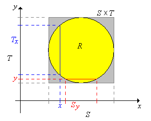
We continue the discussion of multivariate uniform distributions. Suppose that \(j, \, k \in \N_+\) and that \(X\) takes values in \(\R^j\), \(Y\) takes values in \(\R^k\), and \((X, Y)\) is uniformly distributed on a set \(R \in \ms R_{j+k}\) with \(0 \lt \lambda_{j + k}(R) \lt \infty \). The joint probability density function \( f \) of \((X, Y)\) is given by \( f(x, y) = 1 \big/ \lambda_{j + k}(R) \) for \( (x, y) \in R \). Recall that uniform distributions always have constant density functions.
Let \(S \in \ms R_j\) and \(T \in \ms R_k \) be the projections of \(R\) onto \(\R^j\) and \(\R^k\) respectively. Note that \(R \subseteq S \times T\) so \(X\) takes values in \(S\) and \(Y\) takes values in \(T\). For \(x \in S\) let \(T_x \in \ms R_k \) denote the cross sections of \(R\) at \(x\), and for \(y \in T\) let \(S_y \in \ms R_j\) denote the cross section of \(R\) at \(y\). Here are the formal definitions and a picture in the case \(j = k = 1\). \begin{align*} S = \left\{x \in \R^j: (x, y) \in R \text{ for some } y \in \R^k\right\}, & \; T = \left\{y \in \R^k: (x, y) \in R \text{ for some } x \in \R^j\right\}\\ T_x = \{t \in T: (x, t) \in R\}, & \; S_y = \{s \in S: (s, y) \in R\} \end{align*}
In the last section, we saw that even though \((X, Y)\) is uniformly distributed, the marginal distributions of \(X\) and \(Y\) are not uniform in general. However, as the next result shows, the conditional distributions are always uniform.
Suppose that \( (X, Y) \) is uniformly distributed on \( R \). Then
The results are symmetric, so we will prove (a). Recall that \( X \) has probability density function \(g\) given by \[ g(x) = \int_{T_x} f(x, y) \, dy = \int_{T_x} \frac{1}{\lambda_{j+k}(R)} \, dy = \frac{\lambda_k(T_x)}{\lambda_{j+k}(R)}, \quad x \in S \] Hence for \( x \in S \), the conditional probability density function of \( Y \) given \( X = x \) is \[ h(y \mid x) = \frac{f(x, y)}{g(x)} = \frac{1}{\lambda_k(T_x)}, \quad y \in T_x \] and this is the probability density function of the uniform distribution on \( T_x \).
Find the conditional density of each variable given a value of the other, and determine if the variables are independent, in each of the following cases:
The conditional probability density function of \(X\) given \(Y = y\) is denoted \(x \mapsto g(x \mid y)\). The conditional probability density function of \(Y\) given \(X = x\) is denoted \(y \mapsto h(y \mid x)\).
In the bivariate uniform experiment, run the simulation 1000 times in each of the following cases. Watch the points in the scatter plot and the graphs of the marginal distributions.
Suppose that \((X, Y, Z)\) is uniformly distributed on \(R = \{(x, y, z) \in \R^3: 0 \lt x \lt y \lt z \lt 1\}\).
The subscripts 1, 2, and 3 correspond to the variables \( X \), \( Y \), and \( Z \), respectively. Note that the conditions on \((x, y, z)\) in each case are those in the definition of the domain \(R\). They are stated differently to emphasize the domain of the conditional probability density function as opposed to the given values, which function as parameters. Note also that each distribution is uniform on the appropriate region.
Recall the previous discussion of the multivariate hypergeometric distribution. As in that discussion, suppose that a population consists of \(m\) objects, and that each object is one of four types. There are \(a\) objects of type 1, \(b\) objects of type 2, and \(c\) objects of type 3, and \(m - a - b - c\) objects of type 0. We sample \(n\) objects from the population at random, and without replacement. The parameters \(a\), \(b\), \(c\), and \(n\) are nonnegative integers with \(a + b + c \le m\) and \(n \le m\). Denote the number of type 1, 2, and 3 objects in the sample by \(X\), \(Y\), and \(Z\), respectively. Hence, the number of type 0 objects in the sample is \(n - X - Y - Z\). In the following exercises, \(x, \, y, \, z \in \N\).
Suppose that \(z \le c\) and \(n - m + c \le z \le n\). Then the conditional distribution of \((X, Y)\) given \(Z = z\) is hypergeometric, and has the probability density function defined by \[ g(x, y \mid z) = \frac{\binom{a}{x} \binom{b}{y} \binom{m - a - b - c}{n - x - y - z}}{\binom{m - c}{n - z}}, \quad x + y \le n - z\]
This result can be proved analytically but a combinatorial argument is better. The essence of the argument is that we are selecting a random sample of size \(n - z\) without replacement from a population of size \(m - c\), with \(a\) objects of type 1, \(b\) objects of type 2, and \(m - a - b\) objects of type 0. The conditions on \(z\) ensure that \(\P(Z = z) \gt 0\), or equivalently, that the new parameters make sense.
Suppose that \(y \le b\), \(z \le c\), and \(n - m + b \le y + z \le n\). Then the conditional distribution of \(X\) given \(Y = y\) and \(Z = z\) is hypergeometric, and has the probability density function defined by \[ g(x \mid y, z) = \frac{\binom{a}{x} \binom{m - a - b - c}{n - x - y - z}}{\binom{m - b - c}{n - y - z}}, \quad x \le n - y - z\]
Again, this result can be proved analytically, but a combinatorial argument is better. The essence of the argument is that we are selecting a random sample of size \(n - y - z\) from a population of size \(m - b - c\), with \(a\) objects of type 1 and \(m - a - b - c\) objects type 0. The conditions on \(y\) and \(z\) ensure that \(\P(Y = y, Z = z) \gt 0\), or equivalently that the new parameters make sense.
These results generalize in a completely straightforward way to a population with any number of types. In brief, if a random vector has a hypergeometric distribution, then the conditional distribution of some of the variables, given values of the other variables, is also hypergeometric. Moreover, it is clearly not necessary to remember the hideous formulas in the previous two theorems. You just need to recognize the problem as sampling without replacement from a multi-type population, and then identify the number of objects of each type and the sample size. The hypergeometric distribution and the multivariate hypergeometric distribution are studied in more detail in the chapter on finite sampling models.
In a population of 150 voters, 60 are democrats and 50 are republicans and 40 are independents. A sample of 15 voters is selected at random, without replacement. Let \(X\) denote the number of democrats in the sample and \(Y\) the number of republicans in the sample. Give the probability density function of each of the following:
Recall that a bridge hand consists of 13 cards selected at random and without replacement from a standard deck of 52 cards. Let \(X\), \(Y\), and \(Z\) denote the number of spades, hearts, and diamonds, respectively, in the hand. Find the probability density function of each of the following:
Recall the previous discussion of multinomial trials. As in that discussion, suppose that we have a sequence of \(n\) independent trials, each with 4 possible outcomes. On each trial, outcome 1 occurs with probability \(p\), outcome 2 with probability \(q\), outcome 3 with probability \(r\), and outcome 0 with probability \(1 - p - q - r\). The parameters \(p, \, q, \, r \in (0, 1)\), with \(p + q + r \lt 1\), and \(n \in \N_+\). Denote the number of times that outcome 1, outcome 2, and outcome 3 occurs in the \(n\) trials by \(X\), \(Y\), and \(Z\) respectively. Of course, the number of times that outcome 0 occurs is \(n - X - Y - Z\). In the following exercises, \(x, \, y, \, z \in \N\).
For \(z \le n\), the conditional distribution of \((X, Y)\) given \(Z = z\) is also multinomial, and has the probability density function.
\[ g(x, y \mid z) = \binom{n - z}{x, \, y} \left(\frac{p}{1 - r}\right)^x \left(\frac{q}{1 - r}\right)^y \left(1 - \frac{p}{1 - r} - \frac{q}{1 - r}\right)^{n - x - y - z}, \quad x + y \le n - z\]This result can be proved analytically, but a probability argument is better. First, let \( I \) denote the outcome of a generic trial. Then \( \P(I = 1 \mid I \ne 3) = \P(I = 1) / \P(I \ne 3) = p \big/ (1 - r) \). Similarly, \( \P(I = 2 \mid I \ne 3) = q \big/ (1 - r) \) and \( \P(I = 0 \mid I \ne 3) = (1 - p - q - r) \big/ (1 - r) \). Now, the essence of the argument is that effectively, we have \(n - z\) independent trials, and on each trial, outcome 1 occurs with probability \(p \big/ (1 - r)\) and outcome 2 with probability \(q \big/ (1 - r)\).
For \(y + z \le n\), the conditional distribution of \(X\) given \(Y = y\) and \(Z = z\) is binomial, with the probability density function
\[ h(x \mid y, z) = \binom{n - y - z}{x} \left(\frac{p}{1 - q - r}\right)^x \left(1 - \frac{p}{1 - q - r}\right)^{n - x - y - z},\quad x \le n - y - z\]Again, this result can be proved analytically, but a probability argument is better. As before, let \( I \) denote the outcome of a generic trial. Then \( \P(I = 1 \mid I \notin \{2, 3\}) = p \big/ (1 - q - r) \) and \( \P(I = 0 \mid I \notin \{2, 3\}) = (1 - p - q - r) \big/ (1 - q - r) \). Thus, the essence of the argument is that effectively, we have \(n - y - z\) independent trials, and on each trial, outcome 1 occurs with probability \(p \big/ (1 - q - r)\).
These results generalize in a completely straightforward way to multinomial trials with any number of trial outcomes. In brief, if a random vector has a multinomial distribution, then the conditional distribution of some of the variables, given values of the other variables, is also multinomial. Moreover, it is clearly not necessary to remember the specific formulas in the previous two exercises. You just need to recognize a problem as one involving independent trials, and then identify the probability of each outcome and the number of trials. The binomial distribution and the multinomial distribution are studied in more detail in the chapter on Bernoulli trials.
Suppose that peaches from an orchard are classified as small, medium, or large. Each peach, independently of the others is small with probability \(\frac{3}{10}\), medium with probability \(\frac{1}{2}\), and large with probability \(\frac{1}{5}\). In a sample of 20 peaches from the orchard, let \(X\) denote the number of small peaches and \(Y\) the number of medium peaches. Give the probability density function of each of the following:
For a certain crooked, 4-sided die, face 1 has probability \(\frac{2}{5}\), face 2 has probability \(\frac{3}{10}\), face 3 has probability \(\frac{1}{5}\), and face 4 has probability \(\frac{1}{10}\). Suppose that the die is thrown 50 times. Let \(X\), \(Y\), and \(Z\) denote the number of times that scores 1, 2, and 3 occur, respectively. Find the probability density function of each of the following:
The joint distributions in exericse and exercise below are examples of bivariate normal distributions. The conditional distributions are also normal, an important property of the bivariate normal distribution. In general, normal distributions are widely used to model physical measurements subject to small, random errors.
Suppose that \((X, Y)\) has the bivariate normal distribution with probability density function \(f\) defined by \[f(x, y) = \frac{1}{12 \pi} \exp\left[-\left(\frac{x^2}{8} + \frac{y^2}{18}\right)\right], \quad (x, y) \in \R^2\]
Suppose that \((X, Y)\) has the bivariate normal distribution with probability density function \(f\) defined by \[f(x, y) = \frac{1}{\sqrt{3} \pi} \exp\left[-\frac{2}{3} (x^2 - x y + y^2)\right], \quad (x, y) \in \R^2\]