In this section, we will discuss independence, one of the fundamental concepts in probability theory. Independence is frequently invoked as a modeling assumption, and moreover, (classical) probability itself is based on the idea of independent replications of the experiment. Conditional probability is an important prerequisite for this section, but as usual, if you are a new student of probability, you may want to ignore the measure-theoretic details.
Basic Theory
As usual, our starting point is a random experiment modeled by a probability space \( (S, \ms S, \P) \). So to review, \( S \) is the set of outcomes, \( \ms S \) the collection of events, and \( \P \) the probability measure on the sample space \((S, \ms S)\). We will define independence for two events, then for collections of events, and then for collections of random variables. In each case, the basic idea is the same.
Independence of Two Events
Events \(A\) and \(B\) are independent if \(\P(A \cap B) = \P(A) \P(B)\).
If both of the events have positive probability, then independence is equivalent to the statement that the conditional probability of one event given the other is the same as the (unconditional) probability of the event. That is,
\[\P(A \mid B) = \P(A) \iff \P(B \mid A) = \P(B) \iff \P(A \cap B) = \P(A) \P(B)\]
This is how you should think of independence: knowledge that one event has occurred does not change the probability assigned to the other event. Independence of two event was studied in the last section in the context of correlation. In particular, for two events, independent and uncorrelated mean the same thing.
The terms independent and disjoint sound vaguely similar but they are actually very different. First, note that disjointness is a purely set-theory concept while independence is a probability (measure-theoretic) concept. Indeed, two events can be independent relative to one probability measure and dependent relative to another. But most importantly, two disjoint events can never be independent, except in the trivial case that one of the events is null.
Suppose that \(A\) and \(B\) are disjoint events, each with positive probability. Then \(A\) and \(B\) are dependent, and in fact are negatively correlated.
Details:
Note that \(\P(A \cap B) = \P(\emptyset) = 0\) but \(\P(A) \P(B) \gt 0\).
If \(A\) and \(B\) are independent events then intuitively it seems clear that any event that can be constructed from \(A\) should be independent of any event that can be constructed from \(B\). This is the case, as the next result shows. Moreover, this basic idea is essential for the generalization of independence that we will consider shortly.
If \(A\) and \(B\) are independent events, then the following pairs of events are independent:
\(A^c\), \(B\)
\(B\), \(A^c\)
\(A^c\), \(B^c\)
Details:
Suppose that \( A \) and \( B \) are independent. Then by the difference rule and the complement rule,
\[ \P(A^c \cap B) = \P(B) - \P(A \cap B) = \P(B) - \P(A) \, \P(B) = \P(B)\left[1 - \P(A)\right] = \P(B) \P(A^c) \]
Hence \( A^c \) and \( B \) are equivalent. Parts (b) and (c) follow from (a).
An event that is essentially deterministic, that is, has probability 0 or 1, is independent of any other event, even itself.
Suppose that \(A\) and \(B\) are events.
If \(\P(A) = 0\) or \(\P(A) = 1\), then \(A\) and \(B\) are independent.
\(A\) is independent of itself if and only if \(\P(A) = 0\) or \(\P(A) = 1\).
Details:
Recall that if \( \P(A) = 0 \) then \( \P(A \cap B) = 0 \), and if \( \P(A) = 1 \) then \( \P(A \cap B) = \P(B) \). In either case we have \( \P(A \cap B) = \P(A) \P(B) \).
The independence of \( A \) with itself gives \( \P(A) = [\P(A)]^2 \) and hence either \( \P(A) = 0 \) or \( \P(A) = 1 \).
General Independence of Events
To extend the definition of independence to more than two events, we might think that we could just require pairwise independence, the independence of each pair of events. However, this is not sufficient for the strong type of independence that we have in mind. For example, suppose that we have three events \(A\), \(B\), and \(C\). Mutual independence of these events should not only mean that each pair is independent, but also that an event that can be constructed from \(A\) and \(B\) (for example \(A \cup B^c\)) should be independent of \(C\). Pairwise independence does not achieve this. Exercise gives a counterexample with three events that are pairwise independent, but the intersection of two of the events is related to the third event in the strongest possible sense.
Another possible generalization would be to simply require the probability of the intersection of the events to be the product of the probabilities of the events. However, this condition does not even guarantee pairwise independence. Exericse gives a counterexample. However, the definition of independence for two events does generalize in a natural way to an arbitrary collection of events.
Suppose that \( A_i \) is an event for each \( i \) in a nonempty index set \( I \). Then the collection \( \ms A = \{A_i: i \in I\} \) is independent if for every finite \( J \subseteq I \),
\[\P\left(\bigcap_{j \in J} A_j \right) = \prod_{j \in J} \P(A_j)\]
Independence of a collection of events is much stronger than mere pairwise independence of the events in the collection. The basic inheritance property in below follows immediately from the definition.
Suppose that \(\ms A\) is a collection of events.
If \(\ms A\) is independent, then \(\ms B\) is independent for every \(\ms B \subseteq \ms A\).
If \(\ms B\) is independent for every finite \(\ms B \subseteq \ms A\) then \(\ms A\) is independent.
For a finite collection of events, the number of conditions required for mutual independence grows exponentially with the number of events.
For \(n \in \N_+\), there are \(2^n - n - 1\) non-trivial conditions in the definition of the independence of \(n\) events.
Explicitly give the 4 conditions that must be satisfied for events \(A\), \(B\), and \(C\) to be independent.
Explicitly give the 11 conditions that must be satisfied for events \(A\), \(B\), \(C\), and \(D\) to be independent.
Details:
There are \( 2^n \) subcollections of the \( n \) events. One is empty and \( n \) involve a single event. The remaining \( 2^n - n - 1 \) subcollections involve two or more events and correspond to non-trivial conditions.
\(A\), \(B\), \(C\) are independent if and only if
\begin{align*}
& \P(A \cap B) = \P(A) \P(B)\\
&\P(A \cap C) = \P(A) \P(C)\\
& \P(B \cap C) = \P(B) \P(C)\\
& \P(A \cap B \cap C) = \P(A) \P(B) \P(C)
\end{align*}
\(A\), \(B\), \(C\), \(D\) are independent if and only if
\begin{align*}
& \P(A \cap B) = \P(A) \P(B)\\
& \P(A \cap C) = \P(A) \P(C)\\
& \P(A \cap D) = \P(A) \P(D)\\
& \P(B \cap C) = \P(B) \P(C)\\
& \P(B \cap D) = \P(B) \P(D)\\
& \P(C \cap D) = \P(C) \P(D)\\
& \P(A \cap B \cap C) = \P(A) \P(B) \P(C)\\
& \P(A \cap B \cap D) = \P(A) \P(B) \P(D)\\
& \P(A \cap C \cap D) = \P(A) \P(C) \P(D) \\
& \P(B \cap C \cap D) = \P(B) \P(C) \P(D)\\
& \P(A \cap B \cap C \cap D) = \P(A) \P(B) \P(C) \P(D)
\end{align*}
If the events \( A_1, A_2, \ldots, A_n \) are independent, then it follows immediately from the definition that
\[\P\left(\bigcap_{i=1}^n A_i\right) = \prod_{i=1}^n \P(A_i)\]
This is known as the multiplication rule for independent events. Compare this with the general multiplication rule for conditional probability.
The collection of essentially deterministic events \(\ms D = \{A \in \ms S: \P(A) = 0 \text{ or } \P(A) = 1\}\) is independent.
Details:
Suppose that \(n \in \N_+\) and that \( \{A_1, A_2, \ldots, A_n\} \subseteq \ms D \). If \( \P(A_i) = 0 \) for some \( i \in \{1, 2, \ldots, n\} \) then \( \P(A_1 \cap A_2 \cap \cdots \cap A_n) = 0 \). If \( \P(A_i) = 1 \) for every \( i \in \{1, 2, \ldots, n\} \) then \( \P(A_1 \cap A_2 \cap \cdots \cap A_n) = 1 \). In either case,
\[ \P(A_1 \cap A_2 \cdots \cap A_n) = \P(A_1) \P(A_2) \cdots \P(A_n) \]
The next result generalizes on the complements of two independent events.
Suppose that \( \ms A = \{A_i: i \in I\} \) and \( \ms B = \{B_i: i \in I\} \) are two collections of events with the property that for each \( i \in I \), either \( B_i = A_i \) or \( B_i = A_i^c \). Then \( \ms A \) is independent if and only if \( \ms B \) is independent.
Details:
The proof is actually very similar to the proof for two events in , except for more complicated notation. First, by the symmetry of the relation between \( \ms A \) and \( \ms B \), it suffices to show \( \ms A \) indpendent implies \( \ms B \) independent. Next, by , it suffices to consider the case where the index set \( I \) is finite.
Fix \( k \in I \) and define \( B_k = A_k^c \) and \( B_i = A_i \) for \( i \in I \setminus \{k\} \). Suppose now that \( J \subseteq I \). If \( k \notin J \) then trivially, \( \P\left(\bigcap_{j \in J} B_j\right) = \prod_{j \in J} \P(B_j) \). If \( k \in J \), then using the difference rule,
\begin{align*}
\P\left(\bigcap_{j \in J} B_j\right) &= \P\left(\bigcap_{j \in J \setminus \{k\}} A_j\right) - \P\left(\bigcap_{j \in J} A_j\right) \\
& = \prod_{j \in J \setminus\{k\}} \P(A_j) - \prod_{j \in J} \P(A_j) = \left[\prod_{j \in J \setminus\{k\}} \P(A_j)\right][1 - \P(A_k)] = \prod_{j \in J} \P(B_j)
\end{align*}
Hence \( \{B_i: i \in I\} \) is a collection of independent events.
Suppose now that \( \ms B = \{B_i: i \in I\} \) is a general collection of events where \( B_i = A_i \) or \( B_i = A_i^c \) for each \( i \in I \). Then \( \ms B \) can be obtained from \( \ms A \) by a finite sequence of complement changes of the type in (a), each of which preserves independence.
Theorem in turn leads to the type of strong independence that we want. The following exercise gives examples.
If \(A\), \(B\), \(C\), and \(D\) are independent events, then
\(A \cup B\), \(C^c\), \(D\) are independent.
\(A \cup B^c\), \(C^c \cup D^c\) are independent.
Details:
We will give proofs that use the complement theorem in , but to do so, some additional notation is helpful. If \( E \) is an event, let \( E^1 = E \) and \( E^0 = E^c\).
Note that \( A \cup B = \bigcup_{(i, j) \in I} A^i \cap B^j \) where \( I = \{(1, 0), (0, 1), (1, 1)\} \) and note that the events in the union are disjoint. By the distributive property, \( (A \cup B) \cap C^c = \bigcup_{(i, j) \in I} A^i \cap B^j \cap C^0 \) and again the events in the union are disjoint. By additivity and ,
\[ \P[(A \cup B) \cap C^c] = \sum_{(i, j) \in I} \P(A^i) \P(B^j) \P(C^0) = \left(\sum_{(i,j) \in I} \P(A^i) \P(B^j)\right) \P(C^0) = \P(A \cup B) \P(C^c) \]
By exactly the same type of argument, \( \P[(A \cup B) \cap D] = \P(A \cup B) \P(D) \) and \(\P[(A \cup B) \cap C^c \cap D] = \P(A \cup B) \P(C^c) \P(D) \). Directly from , \( \P(C^c \cap D) = \P(C^c) \P(D) \).
Note that \( A \cup B^c = \bigcup_{(i, j) \in I} A^i \cap B^j \) where \( I = \{(0, 0), (1, 0), (1, 1)\} \) and note that the events in the union are disjoint. Similarly \( C^c \cup D^c = \bigcup_{(k, l) \in J} C^i \cap D^j\) where \( J = \{(0, 0), (1, 0), (0, 1)\} \), and again the events in the union are disjoint. By the distributive rule for set operations,
\[ (A \cup B^c) \cap (C^c \cup D^c) = \bigcup_{(i, j, k ,l) \in I \times J} A^i \cap B^j \cap C^k \cap D^l \]
and once again, the events in the union are disjoint. By additivity and ,
\[ \P[(A \cup B^c) \cap (C^c \cup D^c)] = \sum_{(i, j, k ,l) \in I \times J} \P(A^i ) \P(B^j) \P(C^k) \P(D^l) \]
But also by additivity, , and the distributive property of arithmetic,
\[ \P(A \cup B^c) \P(C^c \cup D^c) = \left(\sum_{(i,j) \in I} \P(A^i) \P(B^j)\right) \left(\sum_{(k,l) \in J} \P(C^k) \P(D^l)\right) = \sum_{(i, j, k ,l) \in I \times J} \P(A^i ) \P(B^j) \P(C^k) \P(D^l) \]
The complete generalization of these results is a bit complicated, but roughly means that if we start with a collection of indpendent events, and form new events from disjoint subcollections (using the set operations of union, intersection, and complment), then the new events are independent. The importance of lies in the fact that any event that can be defined in terms of a finite collection of events \( \{A_i: i \in I\} \) can be written as a disjoint union of events of the form \( \bigcap_{i \in I} B_i \) where \( B_i = A_i \) or \( B_i = A_i^c\) for each \( i \in I \).
Another consequence of is a formula for the probability of the union of a collection of independent events that is much nicer than the inclusion-exclusion formula.
If \( A_1, A_2, \ldots, A_n \) are independent events, then
\[\P\left(\bigcup_{i=1}^n A_i\right) = 1 - \prod_{i=1}^n \left[1 - \P(A_i)\right]\]
Details:
From De Morgan's law and the independence of \( A_1^c, A_2^c, \ldots, A_n^c \) we have
\[ \P\left(\bigcup_{i=1}^n A_i \right) = 1 - \P\left( \bigcap_{i=1}^n A_i^c \right) = 1 - \prod_{i=1}^n \P(A_i^c) = 1 - \prod_{i=1}^n \left[1 - \P(A_i)\right] \]
Independence of Random Variables
Suppose now that \((T, \ms T)\) is another measurable space so that \(T\) is a set and \(\ms T\) is a \(\sigma\)-algebra of subsets of \(T\) (the admissible subsets of \(T\)). Recall that a random variable with values in \(T\) is a measurable function from \(S\) to \(T\), so that \(\{X \in A\} \in \ms S\) for every \(A \in \ms T\). In words, a meaningful statment about \(X\) is an event. Intuitively, random variables are independent if information about some of the variables tells us nothing about the other variables. Mathematically, independence of random variables can be reduced to the independence of events. We start with two random variables, where the notation is simplest.
Suppose that \((T, \ms T)\) and \((U, \ms U)\) are measurable spaces and that \(X\) and \(Y\) are random variables with values in \(T\) and \(U\), respectively. Then \(X\) and \(Y\) are independent if
\[\P(X \in A, Y \in B) = \P(X \in A) \P(Y \in B), \quad A \in \ms T, \, B \in \ms U\]
That is, \(X\) and \(Y\) are independent if the events \(\{X \in A\}\) and \(\{Y \in B\}\) are independent for every \(A \in \ms T\) and \(B \in \ms U\). The generalization to arbitrary collections of random variables is straightforward; only the notation is more complicated.
Suppose that \((T_i, \ms T_i)\) is a measurable space for each \(i\) in a nonempty index set \(I\) and that \(X_i\) is a random variable with values in \(T_i\) for each \(i \in I\). The collection of random variables \( \ms X = \{X_i: i \in I\} \) is independent if the collection of events \( \left\{\{X_i \in A_i\}: i \in I\right\} \) is independent for every choice of \( A_i \in \ms T_i \) for \( i \in I \). Equivalently then, \( \ms X \) is independent if for every finite \(J \subseteq I\), and for every choice of \(A_j \in \ms T_j\) for \(j \in J\) we have
\[\P\left(\bigcap_{j \in J} \{X_j \in A_j\} \right) = \prod_{j \in J} \P(X_j \in A_j)\]
Theorem is the inheritance property for independent random variables, analogous to for random variables:
Suppose that \(\ms X\) is a collection of random variables.
If \(\ms X\) is independent, then \(\ms Y\) is independent for every \(\ms Y \subseteq \ms X\)
If \(\ms Y\) is independent for every finite \(\ms Y \subseteq \ms X\) then \(\ms X\) is independent.
It would seem almost obvious that if a collection of random variables is independent, and we transform each variable in deterministic way, then the new collection of random variables should still be independent.
In the setting of definition , suppose now that \((U_i, \ms U_i)\) is another measurable space for \(i \in I\) and that \( g_i \) is a measurable function from \( T_i \) into a \( U_i \) for each \( i \in I \). If \( \{X_i: i \in I\} \) is independent, then \( \{g_i(X_i): i \in I\} \) is also independent.
Details:
Except for the abstract setting, the proof of independence is easy. Suppose that \( A_i \in \ms U_i\) for each \( i \in I \). Then \( \left\{g_i(X_i) \in A_i\right\} = \left\{X_i \in g_i^{-1}(A_i)\right\} \) for \( i \in I \). Since the functions are measurable, \(g^{-1} (A_i) \in \ms T_i\) for \(i \in I\) and then by the independence of \(\{X_i: i \in I\}\), the collection of events \( \left\{\left\{X_i \in g_i^{-1}(A_i)\right\}: i \in I\right\}\) is independent.
Suppose that \((T, \ms T)\) is a measurable space and that \(X\) is a random variable for the experiment with values in \(T\).
\(X\) is independent of itself if and only if \(\P(X \in A) = 0\) or \(\P(X \in A) = 1\) for every \(A \in \ms T\).
If \(X\) is independent of itself then \(X\) is independent of any other random variable \(Y\) for the experiment.
Proof;
The results follow immediately from the corresponding results for events in .
A constant random variable is independent of itself, and hence independent of any other random variable. To make this statement precies, suppose that \((T, \ms T)\) is a measurable spaces and that \(\{x\} \in \ms T\) for every \(x \in T\), a condition that is satisfied for the usual spaces that arise in applications.
Suppose that \(X\) is a random variables with values in \(T\) and that \(\P(X = x) = 1\) for some \(x \in T\) so that \(X\) is constant with probability 1. Then \(X\) is independent of itself.
Details:
The events associated with \(X\) have probability 0 or 1: If \(A \in \ms T\) then \(\P(X \in A) = \bs 1(x \in A)\). So the result follows from the previous one.
Conversely, under certain conditions, a random variable that is independent of itself must be constant with probability 1. We will return to this point in the more advance section on probability spaces.
As with events, the (mutual) independence of random variables is a very strong property. If a collection of random variables is independent, then any subcollection is also independent. New random variables formed from disjoint subcollections are independent. Here is a simple example
Suppose that \(X\), \(Y\), and \(Z\) are independent real-valued random variables. Then
\(\sin(X)\), \(\cos(Y)\), and \(e^Z\) are independent.
\((X, Y)\) and \(Z\) are independent.
\(X^2 + Y^2\) and \(\arctan(Z)\) are independent.
\(X\) and \(Z\) are independent.
\(Y\) and \(Z\) are independent.
In particular, note that statement (b) in the list above is much stronger than the conjunction of statements (d) and (e). Contrapositively, if \(X\) and \(Z\) are dependent, then \((X, Y)\) and \(Z\) are also dependent. Independence of random variables subsumes independence of events.
A collection of events \(\ms A\) is independent if and only if the corresponding collection of indicator variables \(\left\{\bs{1}_A: A \in \ms A\right\}\) is independent.
Details:
Let \( \ms A = \{A_i: i \in I\} \) where \( I \) is a nonempty index set. For \( i \in I \), the only non-trivial events that can be defined in terms of \( \bs 1_{A_i} \) are \( \left\{\bs 1_{A_i} = 1\right\} = A_i \) and \( \left\{\bs 1_{A_i} = 0\right\} = A_i^c \). So \( \left\{\bs 1_{A_i}: i \in I\right\} \) is independent if and only if every collection of the form \( \{B_i: i \in I\} \) is independent, where for each \( i \in I \), either \( B_i = A_i \) or \( B_i = A_i^c \). But by , this is equivalent to the independence of \( \{A_i: i \in I\} \).
Many of the concepts that we have been using informally can now be made precise. A compound experiment that consists of independent stages is essentially just an experiment whose outcome is a sequence of independent random variables \(\bs X = (X_1, X_2, \ldots)\) where \(X_i\) is the outcome of the \(i\)th stage.
In particular, suppose that we have a basic experiment with outcome variable \(X\). By definition, the outcome of the experiment that consists of independent replications of the basic experiment is a sequence of independent random variables \(\bs X = (X_1, X_2, \ldots)\) each with the same probability distribution as \(X\). This is fundamental to the very concept of probability, as expressed in the law of large numbers. From a statistical point of view, suppose that we have a population of objects and a vector of measurements \(X\) of interest for the objects in the sample. The sequence \(\bs X\) above corresponds to sampling from the distribution of \(X\); that is, \(X_i\) is the vector of measurements for the \(i\)th object drawn from the sample. When we sample from a finite population, sampling with replacement generates independent random variables while sampling without replacement generates dependent random variables.
Conditional Independence and Conditional Probability
As noted at the beginning of our discussion, independence of events or random variables depends on the underlying probability measure. Thus, suppose that \(B\) is an event with positive probability. A collection of events or a collection of random variables is conditionally independent given \(B\) if the collection is independent relative to the conditional probability measure \(A \mapsto \P(A \mid B)\). For example, a collection of events \( \{A_i: i \in I\} \) is conditionally independent given \( B \) if for every finite \( J \subseteq I \),
\[\P\left(\bigcap_{j \in J} A_j \biggm| B \right) = \prod_{j \in J} \P(A_j \mid B)\]
Note that the definitions and theorems of this section would still be true, but with all probabilities conditioned on \(B\).
Conversely, conditional probability has a nice interpretation in terms of independent replications of the experiment. Thus, suppose that we start with a basic experiment with \(S\) as the set of outcomes. We let \(X\) denote the outcome random variable, so that mathematically \(X\) is simply the identity function on \(S\). In particular, if \(A\) is an event then trivially, \(\P(X \in A) = \P(A)\). Suppose now that we replicate the experiment independently. This results in a new, compound experiment with a sequence of independent random variables \((X_1, X_2, \ldots)\), each with the same distribution as \(X\). That is, \( X_i \) is the outcome of the \( i \)th repetition of the experiment.
Suppose now that \(A\) and \(B\) are events in the basic experiment with \(\P(B) \gt 0\). In the compound experiment, the event that when \(B\) occurs for the first time, \(A\) also occurs has probability
\[\frac{\P(A \cap B)}{\P(B)} = \P(A \mid B)\]
Details:
In the compound experiment, if we record \( (X_1, X_2, \ldots) \) then the new set of outcomes is \( S^\infty = S \times S \times \cdots \). The event that when \(B\) occurs for the first time, \(A\) also occurs is
\[\bigcup_{n=1}^\infty \left\{X_1 \notin B, X_2 \notin B, \ldots, X_{n-1} \notin B, X_n \in A \cap B\right\}\]
The events in the union are disjoint. Also, since \( (X_1, X_2, \ldots) \) is a sequence of independent variables, each with the distribution of \( X \) we have
\[ \P\left(X_1 \notin B, X_2 \notin B, \ldots, X_{n-1} \notin B, X_n \in A \cap B\right) = \left[\P\left(B^c\right)\right]^{n-1} \P(A \cap B) = \left[1 - \P(B)\right]^{n-1} \P(A \cap B) \]
Hence, using geometric series, the probability of the union is
\[ \sum_{n=1}^\infty \left[1 - \P(B)\right]^{n-1} \P(A \cap B) = \frac{\P(A \cap B)}{1 - \left[1 - \P(B)\right]} = \frac{\P(A \cap B)}{\P(B)} \]
Here is the heuristic argument: Suppose that we create a new experiment by repeating the basic experiment until \(B\) occurs for the first time, and then record the outcome of just the last repetition of the basic experiment. Now the set of outcomes is simply \( B \) and the appropriate probability measure on the new experiment is \(A \mapsto \P(A \mid B)\).
Suppose that \(A\) and \(B\) are disjoint events in a basic experiment with \(\P(A) \gt 0\) and \(\P(B) \gt 0\). In the compound experiment obtained by replicating the basic experiment, the event that \(A\) occurs before \(B\) has probability
\[\frac{\P(A)}{\P(A) + \P(B)}\]
Details:
Note that the event \( A \) occurs before \( B \) is the same as the event when \( A \cup B \) occurs for the first time, \( A \) occurs.
Examples and Applications
Basic Rules
Suppose that \(A\), \(B\), and \(C\) are independent events in an experiment with \(\P(A) = 0.3\), \(\P(B) = 0.4\), and \(\P(C) = 0.8\). Express each of the following events in set notation and find its probability:
\(\P[(A \cap B \cap C^c) \cup (A \cap B^c \cap C) \cup (A^c \cap B \cap C)] = 0.392\)
Suppose that \(A\), \(B\), and \(C\) are independent events for an experiment with \(\P(A) = \frac{1}{3}\), \(\P(B) = \frac{1}{4}\), and \(\P(C) = \frac{1}{5}\). Find the probability of each of the following events:
\((A \cap B) \cup C\)
\(A \cup B^c \cup C\)
\((A^c \cap B^c) \cup C^c\)
Details:
\(\frac{4}{15}\)
\(\frac{13}{15}\)
\(\frac{9}{10}\)
Simple Populations
A small company has 100 employees; 40 are men and 60 are women. There are 6 male executives. How many female executives should there be if gender and rank are independent? The underlying experiment is to choose an employee at random.
Details:
9
Suppose that a farm has four orchards that produce peaches, and that peaches are classified by size as small, medium, and large. The table below gives total number of peaches in a recent harvest by orchard and by size. Fill in the body of the table with counts for the various intersections, so that orchard and size are independent variables. The underlying experiment is to select a peach at random from the farm.
Orchard | Size
Small
Medium
Large
Total
1
400
2
600
3
300
4
700
Total
400
1000
600
2000
Details:
Orchard | Size
Small
Medium
Large
Total
1
80
200
120
400
2
120
300
180
600
3
60
150
90
300
4
140
350
210
700
Total
400
1000
600
2000
Note from exercises and that you cannot see independence in a Venn diagram. Again, independence is a measure-theoretic concept, not a set-theoretic concept.
Bernoulli Trials
A Bernoulli trials sequence is a sequence \(\bs X = (X_1, X_2, \ldots)\) of independent, identically distributed indicator variables. Random variable \(X_i\) is the outcome of trial \(i\), where in the usual terminology of reliability theory, 1 denotes success and 0 denotes failure. The canonical example is the sequence of scores when a coin (not necessarily fair) is tossed repeatedly. Another basic example arises whenever we start with an basic experiment and an event \(A\) of interest, and then repeat the experiment. In this setting, \(X_i\) is the indicator variable for event \(A\) on the \(i\)th run of the experiment. The Bernoulli trials process is named for Jacob Bernoulli, and has a single basic parameter \(p = \P(X_i = 1)\).
If \( X \) is a generic Bernoulli trial, then by definition, \( \P(X = 1) = p \) and \( \P(X = 0) = 1 - p \). Equivalently, \( \P(X = x) = p^x (1 - p)^{1 - x} \) for \( x \in \{0, 1\} \). Thus the result follows by independence.
Note that the sequence of indicator random variables \(\bs X\) is exchangeable. That is, if the sequence \((x_1, x_2, \ldots, x_n)\) in is permuted, the probability does not change. On the other hand, there are exchangeable sequences of indicator random variables that are dependent, as Pólya's urn model so dramatically illustrates.
Let \(Y\) denote the number of successes in the first \(n\) trials. Then
\[\P(Y = y) = \binom{n}{y} p^y (1 - p)^{n-y}, \quad y \in \{0, 1, \ldots, n\}\]
Details:
Note that \( Y = \sum_{i=1}^n X_i \), where \( X_i \) is the outcome of trial \( i \), as in the previous result. For \( y \in \{0, 1, \ldots, n\} \), the event \( \{Y = y\} \) occurs if and only if exactly \( y \) of the \( n \) trials result in success (1). The number of ways to choose the \( y \) trials that result in success is \( \binom{n}{y} \), and by , the probability of any particular sequence of \( y \) successes and \( n - y \) failures is \( p^y (1 - p)^{n-y} \). Thus the result follows by the additivity of probability.
The distribution of \(Y\) is called the binomial distribution with parameters \(n\) and \(p\). More generally, a multinomial trials sequence is a sequence \(\bs X = (X_1, X_2, \ldots)\) of independent, identically distributed random variables, each with values in a finite set \(S\). The canonical example is the sequence of scores when a \(k\)-sided die (not necessarily fair) is thrown repeatedly.
Cards
Consider the experiment that consists of dealing 2 cards at random from a standard deck and recording the sequence of cards dealt. For \(i \in \{1, 2\}\), let \(Q_i\) be the event that card \(i\) is a queen and \(H_i\) the event that card \(i\) is a heart. Compute the appropriate probabilities to verify the following results. Reflect on these results.
In the card experiment, set \(n = 2\). Run the simulation 500 times. For each pair of events in exercise , compute the product of the empirical probabilities and the empirical probability of the intersection. Compare the results.
Dice
Exercise gives three events that are pairwise independent, but not (mutually) independent.
Consider the dice experiment that consists of rolling 2 standard, fair dice and recording the sequence of scores. Let \(A\) denote the event that first score is 3, \(B\) the event that the second score is 4, and \(C\) the event that the sum of the scores is 7. Then
\(A\), \(B\), \(C\) are pairwise independent.
\(A \cap B\) implies (is a subset of) \(C\) and so these events are dependent in the strongest possible sense.
Details:
Note that \( A \cap B = A \cap C = B \cap C = \{(3, 4)\} \), and the probability of the common intersection is \( \frac{1}{36} \). On the other hand, \( \P(A) = \P(B) = \P(C) = \frac{6}{36} = \frac{1}{6} \).
In the dice experiment, set \(n = 2\). Run the experiment 500 times. For each pair of events in exercise , compute the product of the empirical probabilities and the empirical probability of the intersection. Compare the results.
Exercise gives an example of three events with the property that the probability of the intersection is the product of the probabilities, but the events are not pairwise independent.
Suppose that we throw a standard, fair die one time. Let \(A = \{1, 2, 3, 4\}\), \(B = C = \{4, 5, 6\}\). Then
\(\P(A \cap B \cap C) = \P(A) \P(B) \P(C)\).
\(B\) and \(C\) are the same event, and hence are dependent in the strongest possbile sense.
Details:
Note that \( A \cap B \cap C = \{4\} \), so \( \P(A \cap B \cap C) = \frac{1}{6} \). On the other hand, \( \P(A) = \frac{4}{6} \) and \( \P(B) = \P(C) = \frac{3}{6} \).
Suppose that a standard, fair die is thrown 4 times. Find the probability of the following events.
Six does not occur.
Six occurs at least once.
The sum of the first two scores is 5 and the sum of the last two scores is 7.
Details:
\(\left(\frac{5}{6}\right)^4 \approx 0.4823\)
\(1 - \left(\frac{5}{6}\right)^4 \approx 0.5177\)
\(\frac{1}{54}\)
Suppose that a pair of standard, fair dice are thrown 8 times. Find the probability of each of the following events.
Double six does not occur.
Double six occurs at least once.
Double six does not occur on the first 4 throws but occurs at least once in the last 4 throws.
Let \(n, \, k \in \N_+\) and consider the experiment that consists of rolling \(n\) dice, each \(k\)-sided and recording the sequence of scores \(\bs X = (X_1, X_2, \ldots, X_n)\). The following conditions are equivalent (and correspond to the assumption that the dice are fair):
\(\bs X\) is uniformly distributed on \(\{1, 2, \ldots, k\}^n\).
\(\bs X\) is a sequence of independent variables, and \(X_i\) is uniformly distributed on \(\{1, 2, \ldots, k\}\) for each \(i\).
Details:
Let \( S = \{1, 2, \ldots, k\} \) and note that \( S^n \) has \( k^n \) points. Suppose that \( \bs X \) is uniformly distributed on \( S^n \). Then \( \P(\bs X = \bs{x}) = 1 / k^n \) for each \( \bs{x} \in S^n \) so \( \P(X_i = x) = k^{n-1}/k^n = 1 / k \) for each \( x \in S \). Hence \( X_i \) is uniformly distributed on \( S \). Moreover,
\[ \P(\bs X = \bs{x}) = \P(X_1 = x_1) \P(X_2 = x_2) \cdots \P(X_n = x_n), \quad \bs{x} = (x_1, x_2, \ldots, x_n) \in S^n \]
so \( \bs X \) is an independent sequence. Conversely, if \( \bs X \) is an independent sequence and \( X_i \) is uniformly distributed on \( S \) for each \( i \) then \( \P(X_i = x) = 1/k \) for each \( x \in S \) and hence \( \P(\bs X = \bs{x}) = 1/k^n \) for each \( \bs{x} \in S^n \). Thus \( \bs X \) is uniformly distributed on \( S^n \).
A pair of standard, fair dice are thrown repeatedly. Find the probability of each of the following events.
A sum of 4 occurs before a sum of 7.
A sum of 5 occurs before a sum of 7.
A sum of 6 occurs before a sum of 7.
When a sum of 8 occurs the first time, it occurs the hard way as \((4, 4)\).
Details:
\(\frac{3}{9}\)
\(\frac{4}{10}\)
\(\frac{5}{11}\)
\(\frac{1}{5}\)
Problems of the type in exercise are important in the game of craps.
Coins
A biased coin with probability of heads \(\frac{1}{3}\) is tossed 5 times. Let \(\bs X\) denote the outcome of the tosses (encoded as a bit string) and let \(Y\) denote the number of heads. Find each of the following:
\(\P(\bs X = \bs{x})\) for each \(\bs{x} \in \{0, 1\}^5\).
\(\P(Y = y)\) for each \(y \in \{0, 1, 2, 3, 4, 5\}\).
\(\P(1 \le Y \le 3)\)
Details:
\(\frac{32}{243}\) if \(\bs{x} = 00000\), \(\frac{16}{243}\) if \(\bs{x}\) has exactly one 1 (there are 5 of these), \(\frac{8}{243}\) if \(\bs{x}\) has exactly two 1s (there are 10 of these), \(\frac{4}{243}\) if \(\bs{x}\) has exactly three 1s (there are 10 of these), \(\frac{2}{243}\) if \(\bs{x}\) has exactly four 1s (there are 5 of these), \(\frac{1}{243}\) if \(\bs{x} = 11111\)
\(\frac{32}{243}\) if \(y = 0\), \(\frac{80}{243}\) if \(y = 1\), \(\frac{80}{243}\) if \(y = 2\), \(\frac{40}{243}\) if \(y = 3\), \(\frac{10}{243}\) if \(y = 4\), \(\frac{1}{243}\) if \(y = 5\)
\(\frac{200}{243}\)
A box contains a fair coin and a two-headed coin. A coin is chosen at random from the box and tossed repeatedly. Let \(F\) denote the event that the fair coin is chosen, and let \(H_i\) denote the event that toss \(i\) results in heads for \(i \in \N_+\). Then
\((H_1, H_2, \ldots)\) are conditionally independent given \(F\), with \(\P(H_i \mid F) = \frac{1}{2}\) for each \(i\).
\((H_1, H_2, \ldots)\) are conditionally independent given \(F^c\), with \(\P(H_i \mid F^c) = 1\) for each \(i\).
Parts (a) and (b) are essentially modeling assumptions, based on the design of the experiment. If we know what kind of coin we have, then the tosses are independent. Parts (c) and (d) follow by conditioning on the type of coin and using parts (a) and (b). Part (e) follows from (c) and (d). Note that the expression in (d) is not \((3/4)^n\). Part (f) follows from part (d) and Bayes' theorem. Finally part (g) follows from part (f).
Consider again the box in exercise , but we change the experiment as follows: A coin is chosen at random from the box and tossed and the result recorded. The coin is returned to the box and the process is repeated. As before, let \(H_i\) denote the event that toss \(i\) results in heads for \(i \in \N_+\). Then
Again, part (a) is essentially a modeling assumption. Since we return the coin and draw a new coin at random each time, the results of the tosses should be independent. Part (b) follows by conditioning on the type of the \(i\)th coin. Part (c) follows from parts (a) and (b).
Think carefully about the results in exercises and , and the differences between the two models. Tossing a coin produces independent random variables if the probability of heads is fixed (that is, non-random even if unknown). Tossing a coin with a random probability of heads generally does not produce independent random variables; the result of a toss gives information about the probability of heads which in turn gives information about subsequent tosses.
Uniform Distributions
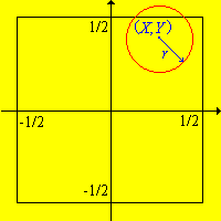
Recall that Buffon's coin experiment consists of tossing a coin with radius \(r \le \frac{1}{2}\) randomly on a floor covered with square tiles of side length 1. The coordinates \((X, Y)\) of the center of the coin are recorded relative to axes through the center of the square in which the coin lands. The following conditions are equivalent:
\((X, Y)\) is uniformly distributed on \(\left[-\frac{1}{2}, \frac{1}{2}\right]^2\).
\(X\) and \(Y\) are independent and each is uniformly distributed on \(\left[-\frac{1}{2}, \frac{1}{2}\right]\).
Buffon's coin experimentDetails:
Let \( S = \left[-\frac{1}{2}, \frac{1}{2}\right] \) so that the square \(S^2\) is the set of outcomes of Buffon's experiment. The standard (Borel) \(\sigma\)-algebra \(\ms S\) of subsets of \(S\) is the one generated by intervals, and so the standard \(\sigma\)-algebra \(\ms S_2\) of subsets of \(S^2\) is the product \(\sigma\)-algebra, generated by rectangles. The standard (Lebesgue) measure \(\lambda_1\) on \((S, \ms S)\) generalizes length, and the standard measure \(\lambda_2\) on \((S^2, \ms S_2)\) is the product measure that generalizes area. Note that \(\lambda_1(S) = \lambda_2(S^2) = 1\). With the technicalities out of the way, suppose that \( (X, Y) \) is uniformly distributed on \( S^2 \), so that \( \P\left[(X, Y) \in C\right] = \lambda_2(C) \) for \( C \in \ms S_2 \). For \( A \in \ms S \),
\[\P(X \in A) = \P\left[(X, Y) \in A \times S\right] = \lambda_2(A \times S) = \lambda_1(A)\]
Hence \( X \) is uniformly distributed on \( S \). By a similar argument, \( Y \) is also uniformly distributed on \( S \). Moreover, for \( A \in \ms S \) and \( B \in \ms S \),
\[ \P(X \in A, Y \in B) = \P[(X, Y) \in A \times B] = \lambda_2(A \times B) = \lambda_1(A) \lambda_1(B) = \P(X \in A) \P(Y \in B) \]
so \( X \) and \( Y \) are independent. Conversely, if \( X \) and \( Y \) are independent and each is uniformly distributed on \( S \), then for \( A \in \ms S \) and \( B \in \ms S \),
\[ \P\left[(X, Y) \in A \times B\right] = \P(X \in A) \P(Y \in B) = \lambda_1(A) \lambda_1(B) = \lambda_2(A \times B) \]
It then follows that \( \P\left[(X, Y) \in C\right] = \lambda_2(C) \) for every \( C \in \ms S_2 \). For more details about this last step, see the section on existence and uniqueness or positive measures.
Compare exercise with exercise on fair dice.
In Buffon's coin experiment, set \(r = 0.3\). Run the simulation 500 times. For the events \(\{X \gt 0\}\) and \(\{Y \lt 0\}\), compute the product of the empirical probabilities and the empirical probability of the intersection. Compare the results.
The arrival time \(X\) of the \(A\) train is uniformly distributed on the interval \((0, 30)\), while the arrival time \(Y\) of the \(B\) train is uniformly distributed on the interval \((15, 30)\). (The arrival times are in minutes, after 8:00 AM). Moreover, the arrival times are independent. Find the probability of each of the following events:
The \(A\) train arrives first.
Both trains arrive sometime after 20 minutes.
Details:
\(\frac{3}{4}\)
\(\frac{2}{9}\)
Reliability
Recall the simple model of structural reliability in which a system is composed of \(n\) components, where \(n \in \N_+\). Suppose in addition that the components operate independently of each other. As before, let \(X_i\) denote the state of component \(i\), where 1 means working and 0 means failure. Thus, our basic assumption is that the state vector \(\bs X = (X_1, X_2, \ldots, X_n)\) is a sequence of independent indicator random variables. We assume that the state of the system (either working or failed) depends only on the states of the components. Thus, the state of the system is an indicator random variable
\[Y = f(X_1, X_2, \ldots, X_n)\]
where \( f: \{0, 1\}^n \to \{0, 1\} \) is the structure function. Generally, the probability that a device is working is the reliability of the device. Thus, we will denote the reliability of component \(i\) by \(p_i = \P(X_i = 1)\) so that the vector of component reliabilities is \(\bs{p} = (p_1, p_2, \ldots, p_n)\). By independence, the system reliability \(r\) is a function of the component reliabilities:
\[r(p_1, p_2, \ldots, p_n) = \P(Y = 1)\]
Appropriately enough, this function is known as the reliability function. Our challenge is usually to find the reliability function \(r\), given the structure function \(f\). When the components all have the same probability \(p\) then of course the system reliability \(r\) is just a function of \(p\). In this case, the state vector \(\bs X = (X_1, X_2, \ldots, X_n)\) forms a sequence of Bernoulli trials as discussed above.
Comment on the independence assumption for real systems, such as your car or your computer.
Recall that a series system is working if and only if each component is working.
The state of the system is \(U = X_1 X_2 \cdots X_n = \min\{X_1, X_2, \ldots, X_n\}\).
The reliability is \(\P(U = 1) = p_1 p_2 \cdots p_n\).
Recall that a parallel system is working if and only if at least one component is working.
The state of the system is \(V = 1 - (1 - X_1)(1 - X_2) \cdots (1 - X_n) = \max\{X_1, X_2, \ldots, X_n\}\).
The reliability is \(\P(V = 1) = 1 - (1 - p_1) (1 - p_2) \cdots (1 - p_n)\).
Recall that a \(k\) out of \(n\) system is working if and only if at least \(k\) of the \(n\) components are working, where \(k \in \{1, 2, \ldots, n\}\). So a parallel system is a 1 out of \(n\) system and a series system is an \(n\) out of \(n\) system. For \(k \in \N_+\), a \(k\) out of \(2 k - 1\) system is a majority rules system. The reliability function of a general \(k\) out of \(n\) system is a mess. However, if the component reliabilities are the same, the function has a reasonably simple form.
For a \(k\) out of \(n\) system with common component reliability \(p\), the system reliability is
\[r(p) = \sum_{i = k}^n \binom{n}{i} p^i (1 - p)^{n - i}\]
Consider a system of 3 independent components with common reliability \(p = 0.8\). Find the reliability of each of the following:
The parallel system.
The 2 out of 3 system.
The series system.
Details:
0.992
0.896
0.512
Consider a system of 3 independent components with reliabilities \(p_1 = 0.8\), \(p_2 = 0.8\), \(p_3 = 0.7\). Find the reliability of each of the following:
The parallel system.
The 2 out of 3 system.
The series system.
Details:
0.994
0.902
0.504
Consider an airplane with an odd number of engines, each with reliability \(p\). Suppose that the airplane is a majority rules system, so that the airplane needs a majority of working engines in order to fly.
Find the reliability of a 3 engine plane as a function of \(p\).
Find the reliability of a 5 engine plane as a function of \(p\).
For what values of \(p\) is a 5 engine plane preferable to a 3 engine plane?
Details:
\(r_3(p) = 3 \, p^2 - 2 \, p^3\)
\(r_5(p) = 6 \, p^5 - 15 \, p^4 + 10 p^3\)
The 5-engine plane would be preferable if \(p \gt \frac{1}{2}\) (which one would hope would be the case). The 3-engine plane would be preferable if \(p \lt \frac{1}{2}\). If \(p = \frac{1}{2}\), the 3-engine and 5-engine planes are equally reliable.
The graph below is known as the Wheatstone bridge network and is named for Charles Wheatstone. The edges represent components, and the system works if and only if there is a working path from vertex \(a\) to vertex \(b\).
A system consists of 3 components, connected in parallel. Because of environmental factors, the components do not operate independently, so our usual assumption does not hold. However, we will assume that under low stress conditions, the components are independent, each with reliability 0.9; under medium stress conditions, the components are independent with reliability 0.8; and under high stress conditions, the components are independent, each with reliability 0.7. The probability of low stress is 0.5, of medium stress is 0.3, and of high stress is 0.2.
Find the reliability of the system.
Given that the system works, find the conditional probability of each stress level.
Details:
0.9917. Condition on the stress level.
0.5037 for low, 0.3001 for medium, 0.1962 for high. Use Bayes' theorem and part (a).
Suppose that bits are transmitted across a noisy communications channel. Each bit that is sent, independently of the others, is received correctly with probability 0.9 and changed to the complementary bit with probability 0.1. Using redundancy to improve reliability, suppose that a given bit will be sent 3 times. We naturally want to compute the probability that we correctly identify the bit that was sent. Assume we have no prior knowledge of the bit, so we assign probability \(\frac{1}{2}\) each to the event that 000 was sent and the event that 111 was sent. Now find the conditional probability that 111 was sent given each of the 8 possible bit strings received.
Details:
Let \(\bs X\) denote the string sent and \(\bs Y\) the string received.
\(\bs{y}\)
\(\P(\bs X = 111 \mid \bs Y = \bs{y})\)
111
\(729/730\)
110
\(9/10\)
101
\(9/10\)
011
\(9/10\)
100
\(1/10\)
010
\(1/10\)
001
\(1/10\)
000
\(1/730\)
Diagnostic Testing
Recall the previous discussion of diagnostic testing. To review, we have an event \(A\) for a random experiment whose occurrence or non-occurrence we cannot observe directly. Suppose now that \(n \in \N_+\) and that we have \(n\) tests for the occurrence of \(A\), labeled from 1 to \(n\). We will let \(T_i\) denote the event that test \(i\) is positive for \(A\).
We assume that the tests are independent in the following sense:
If \(A\) occurs, then \((T_1, T_2, \ldots, T_n)\) are (conditionally) independent and test \(i\) has sensitivity \(a_i = \P(T_i \mid A)\).
If \(A\) does not occur, then \((T_1, T_2, \ldots, T_n)\) are (conditionally) independent and test \(i\) has specificity \(b_i = \P(T_i^c \mid A^c)\).
Note that unconditionally, it is not reasonable to assume that the tests are independent. For example, a positive result for a given test presumably is evidence that the condition \(A\) has occurred, which in turn is evidence that a subsequent test will be positive. In short, we expect that \(T_i\) and \(T_j\) should be positively correlated.
We can form a new, compound test by giving a decision rule in terms of the individual test results. In other words, the event \(T\) that the compound test is positive for \(A\) is a function of \((T_1, T_2, \ldots, T_n)\). The typical decision rules are very similar to the reliability structures in discussed above. A special case of interest is when the \(n\) tests are independent applications of a given basic test. In this case, \(a_i = a\) and \(b_i = b\) for each \(i\).
Consider the compound test that is positive for \(A\) if and only if each of the \(n\) tests is positive for \(A\).
\(T = T_1 \cap T_2 \cap \cdots \cap T_n\)
The sensitivity is \(\P(T \mid A) = a_1 a_2 \cdots a_n\).
The specificity is \(\P(T^c \mid A^c) = 1 - (1 - b_1) (1 - b_2) \cdots (1 - b_n)\)
Consider the compound test that is positive for \(A\) if and only if each at least one of the \(n\) tests is positive for \(A\).
\(T = T_1 \cup T_2 \cup \cdots \cup T_n\)
The sensitivity is \(\P(T \mid A) = 1 - (1 - a_1) (1 - a_2) \cdots (1 - a_n)\).
The specificity is \(\P(T^c \mid A^c) = b_1 b_2 \cdots b_n\).
More generally, we could define the compound \(k\) out of \(n\) test that is positive for \(A\) if and only if at least \(k\) of the individual tests are positive for \(A\) where \(k \in \{1, 2, \ldots, n\}\). The series test in is the \(n\) out of \(n\) test, while the parallel test in is the 1 out of \(n\) test. The \(k\) out of \(2 k - 1\) test is the majority rules test.
Suppose that a woman initially believes that there is an even chance that she is or is not pregnant. She buys three identical pregnancy tests with sensitivity 0.95 and specificity 0.90. Tests 1 and 3 are positive and test 2 is negative.
Find the updated probability that the woman is pregnant.
Can we just say that tests 2 and 3 cancel each other out? Find the probability that the woman is pregnant given just one positive test, and compare the answer with the answer to part (a).
Details:
0.834
No: 0.905.
Suppose that 3 independent, identical tests for an event \(A\) are applied, each with sensitivity \(a \in [0, 1]\) and specificity \(b \in [0, 1]\). Find the sensitivity and specificity of the following tests:
In a criminal trial, the defendant is convicted if and only if all 6 jurors vote guilty. Assume that if the defendant really is guilty, the jurors vote guilty, independently, with probability 0.95, while if the defendant is really innocent, the jurors vote not guilty, independently with probability 0.8. Suppose that 70% of defendants brought to trial are guilty.
Find the probability that the defendant is convicted.
Given that the defendant is convicted, find the probability that the defendant is guilty.
Comment on the assumption that the jurors act independently.
Details:
0.5148
0.99996
The independence assumption is not reasonable since jurors collaborate.
Genetics
Refer to the previous discussion of genetics if you need to review some of the definitions in this section. Recall first that the ABO blood type in humans is determined by three alleles: \(a\), \(b\), and \(o\). Furthermore, \(a\) and \(b\) are co-dominant and \(o\) is recessive. Suppose that in a certain population, the proportion of \(a\), \(b\), and \(o\) alleles are \(p\), \(q\), and \(r\) respectively. Of course we must have \(p \gt 0\), \(q \gt 0\), \(r \gt 0\) and \(p + q + r = 1\).
Suppose that the blood genotype in a person is the result of independent alleles, chosen with probabilities \(p\), \(q\), and \(r\) as above.
The probability distribubtion of the geneotypes is given in the following table:
Genotype
\(aa\)
\(ab\)
\(ao\)
\(bb\)
\(bo\)
oo
Probability
\(p^2\)
\(2 p q\)
\(2 p r\)
\(q^2\)
\(2 q r\)
\(r^2\)
The probability distribution of the blood types is given in the following table:
Blood type
\(A\)
\(B\)
\(AB\)
\(O\)
Probability
\(p^2 + 2 p r\)
\(q^2 + 2 q r\)
\(2 p q\)
\(r^2\)
Details:
Part (a) follows from the independence assumption and basic rules of probability. Even though genotypes are listed as unordered pairs, note that there are two ways that a heterozygous genotype can occur, since either parent could contribute either of the two distinct alleles. Part (b) follows from part (a) and basic rules of probability.
Exercise is related to the Hardy-Weinberg model of genetics. The model is named for the English mathematician Godfrey Hardy and the German physician Wilhelm Weiberg
Suppose that the probability distribution for the set of blood types in a certain population is given in the following table:
Blood type
\(A\)
\(B\)
\(AB\)
\(O\)
Probability
0.360
0.123
0.038
0.479
Find \(p\), \(q\), and \(r\).
Details:
\(p = 0.224\), \(q = 0.084\), \(r = 0.692\)
Suppose next that pod color in certain type of pea plant is determined by a gene with two alleles: \(g\) for green and \(y\) for yellow, and that \(g\) is dominant and \(o\) recessive.
Suppose that 2 green-pod plants are bred together. Suppose further that each plant, independently, has the recessive yellow-pod allele with probability \(\frac{1}{4}\).
Find the probability that 3 offspring plants will have green pods.
Given that the 3 offspring plants have green pods, find the updated probability that both parents have the recessive allele.
Details:
\(\frac{987}{1024}\)
\(\frac{27}{987}\)
Next consider a sex-linked hereditary disorder in humans (such as colorblindness or hemophilia). Let \(h\) denote the healthy allele and \(d\) the defective allele for the gene linked to the disorder. Recall that \(h\) is dominant and \(d\) recessive for women.
Suppose that a healthy woman initially has a \(\frac{1}{2}\) chance of being a carrier. (This would be the case, for example, if her mother and father are healthy but she has a brother with the disorder, so that her mother must be a carrier).
Find the probability that the first two sons of the women will be healthy.
Given that the first two sons are healthy, compute the updated probability that she is a carrier.
Given that the first two sons are healthy, compute the conditional probability that the third son will be healthy.
Details:
\(\frac{5}{8}\)
\(\frac{1}{5}\)
\(\frac{9}{10}\)
Laplace's Rule of Succession
Suppose \(m \in \N_+\) that we have \(m + 1\) coins, labeled \(0, 1, \ldots, m\). Coin \(i\) lands heads with probability \(\frac{i}{m}\) for each \(i \in \{0, 1, \ldots, m\}\). The experiment is to choose a coin at random (so that each coin is equally likely to be chosen) and then toss the chosen coin repeatedly.
For \(n \in \N_+\), the probability that the first \(n\) tosses are all heads is \(p_{m,n} = \frac{1}{m+1} \sum_{i=0}^m \left(\frac{i}{m}\right)^n\)
\(p_{m,n} \to \frac{1}{n+1} \) as \(m \to \infty\)
The conditional probability that toss \(n + 1\) is heads given that the previous \(n\) tosses were all heads is \(\frac{p_{m,n+1}}{p_{m,n}}\)
\(\frac{p_{m,n+1}}{p_{m,n}} \to \frac{n+1}{n+2}\) as \(m \to \infty\)
Details:
Part (a) follows by conditioning on the chosen coin. For part (b), note that \( p_{m,n} \) is an approximating sum for \( \int_0^1 x^n \, dx = \frac{1}{n + 1} \). Part (c) follows from the definition of conditional probability, and part (d) is a trivial consequence of (b), (c).
In exercise , note that coin 0 is two-tailed, the probability of heads increases with \( i \), and coin \(m\) is two-headed. The limiting conditional probability in part (d) is called Laplace's Rule of Succession, named after Simon Laplace. This rule was used by Laplace and others as a general principle for estimating the conditional probability that an event will occur on time \(n + 1\), given that the event has occurred \(n\) times in succession.
Suppose that a missile has had 10 successful tests in a row. Compute Laplace's estimate that the 11th test will be successful. Does this make sense?