The purpose of this section is to study how the distribution of a pair of random variables is related to the distributions of the variables individually. The general setting discussed in the introduction is essential for this section. Even if our interest is only in discrete distribution, continuous distributions on Euclidean spaces, and mixtures of these two types, without the general setting we would need multiple special cases for every result.
We start with a random experiment, modeled by a probability space \((\Omega, \ms F, \P)\). So to review, \(\Omega\) is the set of outcomes, \(\ms F\) is the collection of events, and \(\P\) is the probability measure on the sample subspace \((\Omega, \ms F)\). Suppose now that \((S, \ms S)\) and \((T, \ms T)\) are measurable spaces of the type discussed in the introduction, and that \(X\) and \(Y\) are random variables for the experiment with values in \(S\) and \(T\). As usual, the important special cases are when the spaces are discrete or Euclidean. Recall that the product space is \((S \times T, \ms S \times \ms T)\) where \(\ms S \times \ms T\) is the \(\sigma\)-algebra generated by product sets of the form \(A \times B\) with \(A \in \ms S\) and \(B \in \ms T\). Since \(X\) and \(Y\) are random variables with value in \(S\) and \(T\) respectively, \((X, Y)\) is a random variable with values in \(S \times T\). The purpose of this section is to study how the distribution of \((X, Y)\) is related to the distributions of \(X\) and \(Y\) individually.
Recall that
In this context, the distribution of \((X, Y)\) is called the joint distribution, while the distributions of \(X\) and of \(Y\) are referred to as marginal distributions.
The first rather trivial but important point, is that the marginal distributions can be obtained from the joint distribution.
Note that
The converse does not hold in general. The joint distribution contains much more information than the marginal distributions separately. However, the converse does hold if \(X\) and \(Y\) are independent.
Let \(P\) and \(Q\) denote the probability distributions of \(X\) and \(Y\), respectively. If \(X\) and \(Y\) are independent, then the distribution of \((X, Y)\) is the product probability measure \(P \times Q\).
If \(X\) and \(Y\) are independent then, \[\P\left[(X, Y) \in A \times B\right] = \P(X \in A, Y \in B) = \P(X \in A) \P(Y \in B) = P(A) Q(B), \quad A \in \ms S, \, B \in \ms T \] The unique probability measure that satisfies this condition is the product \(P \times Q\) so it follows that \[\P[(X, Y) \in C] = (P \times Q)(C), \quad C \in \ms S \times \ms T \]
Suppose now that \(\mu\) and \(\nu\) are \(\sigma\)-finite positve measures on \((S, \ms S)\) and \((T, \ms T)\), respectively. Recall that in general, measurable spaces often have natural reference measures associated with them, for example counting measure on discrete spaces and Lebesgue measure on Euclidean spaces. The product measure \(\mu \times \nu\) is the natural measure for \((S \times T, \ms S \times \ms T)\) and is the unique measure that satisfies \[(\mu \times \nu)(A \times B) = \mu(A) \nu(B), \quad A \in \ms S, \, B \in \ms T\] In addition, an integral is associated with each of the positive measure spaces, and the probability distributions of the random variables are often defined in terms of density functions. Recall that a density function exists if and only if the probability distribtion is absolutely continuous with respect to the reference measure, so that a measurable set that has measure 0 must have probability 0. In this case, the probability of a set is simply the integral of the density over that set. Our goal in this discussion is to see how the joint density function of \((X, Y)\) is related to the marginal density functions of \(X\) and \(Y\). Of course, all density functions mentioned are with respect to the corresponding reference measures.
Suppose that \( (X, Y) \) has density function \( f: S \times T \to (0, \infty) \). Then \(X\) and \(Y\) have density functions \(g\) and \(h\) given by \begin{align*} g(x) &= \int_T f(x, y), \, d\nu(y), \quad x \in S\\ h(y) &= \int_S f(x, y), \, d\mu(x), \quad y \in T \end{align*}
The two results are anlaogous, so we prove the first one. Except for the abstraction of using integrals with respect to measures, the proof is very simple. \[\P(X \in A) = \P[(X, Y) \in A \times T] = \int_{A \times T} f(x, y) \, d(\mu \times \nu)(x, y) = \int_A \left(\int_T f(x, y) \, d\nu(y)\right) d\mu(x) = \int_A g(x) d\mu(x), \quad A \in \ms S\] So by the very meaning of the term, \(g\) is a probability density of \(X\). The last step in the displayed equation, writing the integral with respect to the product measure as iterated integrals, is justified by Fubini's theorem, named for Guido Fubini. The use of this theorem is why we need the measures to be \(\sigma\)-finite.
It's easy to see that if \((X, Y)\) is absolutely continuous, then so are \(X\) and \(Y\). For \(X\), note that if \(A \in \ms S\) and \(\mu(A) = 0\) then \((\mu \times \nu)(A \times T) = 0\) and hence \[\P(X \in A) = \P[(X, Y) \in A \times T] = 0\] But this is not required in the proof above.
In the context of this theorems, \(f\) is called the joint probability density function of \((X, Y)\), while \(g\) and \(h\) are called the marginal density functions of \(X\) and of \(Y\), respectively. The term marginal comes from the discrete (in fact finite) case where \(f\) is given in the body of a table and then \(g\) and \(h\) in the margins. You can see this in some of the computational exercises in below.
Conversely however, assuming that \(X\) and \(Y\) have density functions, we cannot recover the density function of \((X, Y)\) (in fact, it may not even exist). Once again, the joint density carries much more information than the marginal densities individually. However when the variables are independent, the joint density is the product of the marginal densities.
Suppose that \(X\) and \(Y\) are independent and have probability density function \( g \) and \( h \) respectively. Then \((X, Y)\) has probability density function \(f\) given by \[f(x, y) = g(x) h(y), \quad (x, y) \in S \times T\]
The main tool is the fact that an event defined in terms of \( X \) is independent of an event defined in terms of \( Y \). \[\P[(X, Y) \in A \times B] = \P(X \in A) \P(Y \in B) = \left(\int_A g(x) \, d\mu(x)\right) \left(\int_B h(y) \, d\nu(y)\right) = \int_{A \times B} h(x) g(y) \, d(\mu \times \nu)(x, y), \quad A \in \ms S, \, B \in \ms T\] The distribution of \((X, Y)\) is completely determined by its values on product sets, so it follows that \[\P[(X, Y) \in C] = \int_C g(x) h(y) \, d(\mu \times \nu)(x, y), \quad C \in \ms S \times \ms T\] Once again, writing the product integral as integral with respect to the product measure is a consequence of Fubini's theorem.
Proposition below gives a converse to . If the joint probability density factors into a function of \(x\) only and a function of \(y\) only, then \(X\) and \(Y\) are independent, and we can almost identify the individual probability density functions just from the factoring.
Factoring Theorem. Suppose that \((X, Y)\) has probability density function \(f\) of the form \[f(x, y) = u(x) v(y), \quad (x, y) \in S \times T\] where \(u: S \to [0, \infty)\) and \(v: T \to [0, \infty)\) are measurable. Then \(X\) and \(Y\) are independent, and there exists a constant \(c \in (0, \infty)\) such that \(X\) and \(Y\) have probability density functions \(g\) and \(h\), respectively, given by \begin{align} g(x) = & c \, u(x), \quad x \in S \\ h(y) = & \frac{1}{c} v(y), \quad y \in T \end{align}
Note that \[ \P(X \in A, Y \in B) = \P\left[(X, Y) \in A \times B\right] = \int_{A \times B} f(x, y) \, d(\mu \times \nu)(x, y) = \int_A u(x) \, d\mu(x) \, \int_B v(y) \, d\nu(y), \quad A \in \ms S, \, B \in \ms T \] Letting \( B = T \) in the displayed equation gives \( \P(X \in A) = \int_A c \, u(x) \, d\mu(x) \) for \( A \in \ms S \), where \( c = \int_T v(y) \, d\nu(y) \). By definition, \( X \) has density \( g = c \, u \). Next, letting \( A = S \) in the displayed equation gives \( \P(Y \in B) = \int_B k \, v(y) \, d\nu(y) \) for \( B \in \ms T \), where \( k = \int_S u(x) \, d\mu(x) \). Thus, \( Y \) has density \( g = k \, v \). Next, letting \( A = S \) and \( B = T \) in the displayed equation gives \( 1 = c \, k \), so \( k = 1 / c \). Now note that the displayed equation holds with \( u \) replaced by \( g \) and \( v \) replaced by \( h \), and this in turn gives \( \P(X \in A, Y \in B) = \P(X \in A) \P(Y \in B) \), so \( X \) and \( Y \) are independent.
The last two results extend in a completely straightforward way to more than two random variables. To set up the notation, suppose that \(n \in \N_+\) and that \((S_i, \ms S_i, \mu_i)\) is a positive measure space for \(i \in \{1, 2, \ldots, n\}\). The product space is \[(S_1 \times S_2 \times \cdots \times S_n, \ms S_1 \times \ms S_2 \times \cdots \times S_n, \mu_1 \times \mu_2 \times \cdots \times \mu_n)\] As always, density functions are with respect to the appropriate reference measures.
Suppose that \(X_i\) is a random variable with values in \(S_i\) and has probability density funcion \(g_i\) for \(i \in \{1, 2, \ldots, n\}\). If the random variables are independent then the random vector \(\bs{X} = (X_1, X_2, \ldots, X_n)\) has probability density function \(f\) given by \[f(x_1, x_2, \ldots, x_n) = g_1(x_1) g_2(x_2) \cdots g_n(x_n), \quad (x_1, x_2, \ldots, x_n) \in S_1 \times S_2 \cdots \times S_n\]
The special case where the distributions are all the same is particularly important. Suppose \((S, \ms S, \mu)\) is a positve measure space.
Suppose that \(\bs{X} = (X_1, X_2, \ldots, X_n)\) is a sequence of independent random variables, each taking values in \(S\) and with common probability density function \(g\). Then \(\bs X\) has probability density function \(f\) given by \[f(x_1, x_2, \ldots, x_n) = g(x_1) g(x_2) \cdots g(x_n), \quad (x_1, x_2, \ldots, x_n) \in S^n\]
In probability jargon, \(\bs X\) is a sequence of independent, identically distributed variables, a phrase that comes up so often that it is often abbreviated as IID. In statistical jargon, \(\bs X\) is a random sample of size \(n\) from the common distribution. As is evident from the special terminology, this situation is very impotant in both branches of mathematics. In statistics, the joint probability density function \(f\) plays an important role in procedures such as maximum likelihood and the identification of uniformly best estimators.
Recall that (mutual) independence of random variables is a very strong property. If a collection of random variables is independent, then any subcollection is also independent. New random variables formed from disjoint subcollections are independent. Here is a simple example:
Suppose that \(X\), \(Y\), and \(Z\) are independent real-valued random variables. Then
In particular, note that statement (b) in the list above is much stronger than the conjunction of statements (e) and (e). Restated, if \(X\) and \(Z\) are dependent, then \((X, Y)\) and \(Z\) are also dependent.
Recall that a standard die is an ordinary six-sided die, with faces numbered from 1 to 6. The answers in the next couple of exercises give the joint distribution in the body of a table, with the marginal distributions literally in the magins. Such tables are the reason for the term marginal distibution.
Suppose that two standard, fair dice are rolled and the sequence of scores \((X_1, X_2)\) recorded. Our ususal assumption is that the variables \(X_1\) and \(X_2\) are independent. Let \(Y = X_1 + X_2\) and \(Z = X_1 - X_2\) denote the sum and difference of the scores, respectively.
Let \(f\) denote the density function of \((Y, Z)\), \(g\) the density function of \(Y\) and \(h\) the density function of \(Z\). The density functions are give in the following table. Random variables \(Y\) and \(Z\) are dependent
| \(f(y, z)\) | \(y = 2\) | 3 | 4 | 5 | 6 | 7 | 8 | 9 | 0 | 11 | 12 | \(h(z)\) |
|---|---|---|---|---|---|---|---|---|---|---|---|---|
| \(z = -5\) | 0 | 0 | 0 | 0 | 0 | \(\frac{1}{36}\) | 0 | 0 | 0 | 0 | 0 | \(\frac{1}{36}\) |
| \(-4\) | 0 | 0 | 0 | 0 | \(\frac{1}{36}\) | 0 | \(\frac{1}{36}\) | 0 | 0 | 0 | 0 | \(\frac{2}{36}\) |
| \(-3\) | 0 | 0 | 0 | \(\frac{1}{36}\) | 0 | \(\frac{1}{36}\) | 0 | \(\frac{1}{36}\) | 0 | 0 | 0 | \(\frac{3}{36}\) |
| \(-2\) | 0 | 0 | \(\frac{1}{36}\) | 0 | \(\frac{1}{36}\) | 0 | \(\frac{1}{36}\) | 0 | \(\frac{1}{36}\) | 0 | 0 | \(\frac{4}{36}\) |
| \(-1\) | 0 | \(\frac{1}{36}\) | 0 | \(\frac{1}{36}\) | 0 | \(\frac{1}{36}\) | 0 | \(\frac{1}{36}\) | 0 | \(\frac{1}{36}\) | 0 | \(\frac{5}{36}\) |
| 0 | \(\frac{1}{36}\) | 0 | \(\frac{1}{36}\) | 0 | \(\frac{1}{36}\) | 0 | \(\frac{1}{36}\) | 0 | \(\frac{1}{36}\) | 0 | \(\frac{1}{36}\) | \(\frac{6}{36}\) |
| 1 | 0 | \(\frac{1}{36}\) | 0 | \(\frac{1}{36}\) | 0 | \(\frac{1}{36}\) | 0 | \(\frac{1}{36}\) | 0 | \(\frac{1}{36}\) | 0 | \(\frac{5}{36}\) |
| 2 | 0 | 0 | \(\frac{1}{36}\) | 0 | \(\frac{1}{36}\) | 0 | \(\frac{1}{36}\) | 0 | \(\frac{1}{36}\) | 0 | 0 | \(\frac{4}{36}\) |
| 3 | 0 | 0 | 0 | \(\frac{1}{36}\) | 0 | \(\frac{1}{36}\) | 0 | \(\frac{1}{36}\) | 0 | 0 | 0 | \(\frac{3}{36}\) |
| 4 | 0 | 0 | 0 | 0 | \(\frac{1}{36}\) | 0 | \(\frac{1}{36}\) | 0 | 0 | 0 | 0 | \(\frac{2}{36}\) |
| 5 | 0 | 0 | 0 | 0 | 0 | \(\frac{1}{36}\) | 0 | 0 | 0 | 0 | 0 | \(\frac{1}{36}\) |
| \(g(y)\) | \(\frac{1}{36}\) | \(\frac{2}{36}\) | \(\frac{3}{36}\) | \(\frac{4}{36}\) | \(\frac{5}{36}\) | \(\frac{6}{36}\) | \(\frac{5}{36}\) | \(\frac{4}{36}\) | \(\frac{3}{36}\) | \(\frac{2}{36}\) | \(\frac{1}{36}\) | 1 |
Suppose that two standard, fair dice are rolled and the sequence of scores \((X_1, X_2)\) recorded. Let \(U = \min\{X_1, X_2\}\) and \(V = \max\{X_1, X_2\}\) denote the minimum and maximum scores, respectively.
Let \(f\) denote the density function of \((U, V)\), \(g\) the density function of \(U\), and \(h\) the density function of \(V\). The density functions are given in the following table. Random variables \(U\) and \(V\) are dependent.
| \(f(u, v)\) | \(u = 1\) | 2 | 3 | 4 | 5 | 6 | \(h(v)\) |
|---|---|---|---|---|---|---|---|
| \(v = 1\) | \(\frac{1}{36}\) | 0 | 0 | 0 | 0 | 0 | \(\frac{1}{36}\) |
| 2 | \(\frac{2}{36}\) | \(\frac{1}{36}\) | 0 | 0 | 0 | 0 | \(\frac{3}{36}\) |
| 3 | \(\frac{2}{36}\) | \(\frac{2}{36}\) | \(\frac{1}{36}\) | 0 | 0 | 0 | \(\frac{5}{36}\) |
| 4 | \(\frac{2}{36}\) | \(\frac{2}{36}\) | \(\frac{2}{36}\) | \(\frac{1}{36}\) | 0 | 0 | \(\frac{7}{36}\) |
| 5 | \(\frac{2}{36}\) | \(\frac{2}{36}\) | \(\frac{2}{36}\) | \(\frac{2}{36}\) | \(\frac{1}{36}\) | 0 | \(\frac{9}{36}\) |
| 6 | \(\frac{2}{36}\) | \(\frac{2}{36}\) | \(\frac{2}{36}\) | \(\frac{2}{36}\) | \(\frac{2}{36}\) | \(\frac{1}{36}\) | \(\frac{11}{36}\) |
| \(g(u)\) | \(\frac{11}{36}\) | \(\frac{9}{36}\) | \(\frac{7}{36}\) | \(\frac{5}{36}\) | \(\frac{3}{36}\) | \(\frac{1}{36}\) | 1 |
Exercise and show clearly how little information is given with the marginal distributions compared to the joint distribution. With the marginal density functions alone, you could not even determine the support set of the joint distribution, let alone the values of the joint density function.
Suppose that \((X, Y)\) has probability density function \(f\) given by \(f(x, y) = x + y\) for \(0 \le x \le 1\), \(0 \le y \le 1\).
Suppose that \((X, Y)\) has probability density function \(f\) given by \(f(x, y) = 2 ( x + y)\) for \(0 \le x \le y \le 1\).
Suppose that \((X, Y)\) has probability density function \(f\) given by \(f(x, y) = 6 x^2 y\) for \(0 \le x \le 1\), \(0 \le y \le 1\).
Exercise is a good illustration of the factoring . Without any work at all, we can tell that the density function of \(X\) is proportional to \(x \mapsto x^2\) on the interval \([0, 1]\), the density function of \(Y\) is proportional to \(y \mapsto y\) on the interval \([0, 1]\), and that \(X\) and \(Y\) are independent. The only thing unclear is how the constant 6 factors.
Suppose that \((X, Y)\) has probability density function \(f\) given by \(f(x, y) = 15 x^2 y\) for \(0 \le x \le y \le 1\).
Note that in , the factoring does not apply. Random variables \(X\) and \(Y\) each take values in \([0, 1]\), but the joint density function factors only on part of \([0, 1]^2\).
Suppose that \((X, Y, Z)\) has probability density function \(f\) given \(f(x, y, x) = 2 (x + y) z\) for \(0 \le x \le 1\), \(0 \le y \le 1\), \(0 \le z \le 1\).
Suppose that \((X, Y)\) has probability density function \(f\) given by \(f(x, y) = 2 e^{-x} e^{-y}\) for \(0 \le x \le y \lt \infty\).
In , \( X \) has an exponential distribution with rate parameter 2. Recall that exponential distributions are widely used to model random times, particularly in the context of the Poisson model.
Suppose that \(X\) and \(Y\) are independent, and that \(X\) has probability density function \(g\) given by \(g(x) = 6 x (1 - x)\) for \(0 \le x \le 1\), and that \(Y\) has probability density function \(h\) given by \(h(y) = 12 y^2 (1 - y)\) for \(0 \le y \le 1\).
In , \( X \) and \( Y \) have beta distributions, which are widely used to model random probabilities and proportions.
Suppose that \(\Theta\) and \(\Phi\) are independent random angles, with common probability density function \(g\) given by \(g(t) = \sin(t)\) for \(0 \le t \le \frac{\pi}{2}\).
The common distribution of \( X \) and \( Y \) in governs a random angle in Bertrand's problem.
Suppose that \(X\) and \(Y\) are independent, and that \(X\) has probability density function \(g\) given by \(g(x) = \frac{2}{x^3}\) for \(1 \le x \lt \infty\), and that \(Y\) has probability density function \(h\) given by \(h(y) = \frac{3}{y^4}\) for \(1 \le y \lt\infty\).
Both \(X\) and \(Y\) in have Pareto distributions, named for Vilfredo Pareto. Pareto distributions are used to model certain economic variables.
Suppose that \((X, Y)\) has probability density function \(g\) given by \(g(x, y) = 15 x^2 y\) for \(0 \le x \le y \le 1\), and that \(Z\) has probability density function \(h\) given by \(h(z) = 4 z^3\) for \(0 \le z \le 1\), and that \((X, Y)\) and \(Z\) are independent.
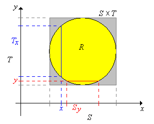
Multivariate uniform distributions give a geometric interpretation of some of the concepts in this section. Recall that \(\ms R^n\) is the \(\sigma\)-algebra of Borel measurable subsets of \(\R^n\) for \(n \in \N_+\) and \(\lambda^n\) is \(n\)-dimesional Lebesgue measure. Suppose now that \(j, \, k \in \N_+\) and that \(X\) takes values in \(\R^j\), \(Y\) takes values in \(\R^k\), and \((X, Y)\) is uniformly distributed on a set \(R \in \ms R_{j+k}\) with \(0 \lt \lambda_{j+k}(R) \lt \infty \). The joint probability density function \( f \) of \((X, Y)\) is given by \( f(x, y) = 1 \big/ \lambda_{j+k}(R) \) for \( (x, y) \in R \). Recall that uniform distributions always have constant density functions. For the discussion that follows, you may need to review projections and cross sections of Cartesian product sets.
Let \(S \in \ms R_j\) and \(T \in \ms R_k \) be the projections of \(R\) onto \(\R^j\) and \(\R^k\) respectively. Note that \(R \subseteq S \times T\) so \(X\) takes values in \(S\) and \(Y\) takes values in \(T\). For \(x \in S\) let \(T_x \in \ms R_k \) denote the cross sections of \(R\) at \(x\), and for \(y \in T\) let \(S_y \in \ms R_j\) denote the cross section of \(R\) at \(y\). Here are the formal definitions and a picture in the case \(j = k = 1\). \begin{align*} S = \left\{x \in \R^j: (x, y) \in R \text{ for some } y \in \R^k\right\}, & \; T = \left\{y \in \R^k: (x, y) \in R \text{ for some } x \in \R^j\right\}\\ T_x = \{t \in T: (x, t) \in R\}, & \; S_y = \{s \in S: (s, y) \in R\} \end{align*}
The probability density functions \(g\) and \( h \) of \(X\) and \( Y \) are proportional to the cross-sectional measures:
From our general theory, \( X \) has density function \( g \) given by \[ g(x) = \int_T f(x, y) \, dy = \int_{T_x} \frac{1}{\lambda_{j+k}(R)} \, dy = \frac{\lambda_k\left(T_x\right)}{\lambda_{j+k}(R)}, \quad x \in S \] The integral is the Lebesgue integral, but recall that this integral agrees with the ordinary Riemann integral of calculus for the type of sets that typically occur in applications. Also, it's technically possible that \(\lambda_k(T_x) = \infty\) for some \(x \in S\), but the set of such \(x\) has measure 0. That is, \(\lambda_j\{x \in S: \lambda_k(T_x) = \infty\} = 0\). The result for \( Y \) is analogous.
In particular, note from previous theorem that \(X\) and \(Y\) are neither independent nor uniformly distributed in general. However, these properties do hold if \(R\) is a Cartesian product set.
Suppose that \(R = S \times T\).
In this case, \( T_x = T \) and \( S_y = S \) for every \( x \in S \) and \( y \in T \). Also, \( \lambda_{j+k}(R) = \lambda_j(S) \lambda_k(T) \), so for \( x \in S \) and \( y \in T \), \( f(x, y) = 1 \big/ [\lambda_j(S) \lambda_k(T)] \), \( g(x) = 1 \big/ \lambda_j(S) \), \( h(y) = 1 \big/ \lambda_k(T) \).
In each of the following cases, find the joint and marginal probabilit density functions, and determine if \(X\) and \(Y\) are independent.
In the following, \(f\) is the density function of \((X, Y)\), \(g\) the density function of \(X\), and \(h\) the density function of \(Y\).
In the bivariate uniform experiment, run the simulation 1000 times for each of the following cases. Watch the points in the scatter plot and the graphs of the marginal distributions. Interpret what you see in the context of the discussion above.
Suppose that \((X, Y, Z)\) is uniformly distributed on the cube \([0, 1]^3\).
Suppose that \((X, Y, Z)\) is uniformly distributed on \(\{(x, y, z): 0 \le x \le y \le z \le 1\}\).
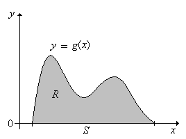
Proposition below shows how an arbitrary continuous distribution can be obtained from a uniform distribution. This result is useful for simulating certain continuous distributions, as we will see. To set up the basic notation, suppose that \(n \in \N_+\) and that \(g\) is a probability density function for a distribution on an \(n\)-dimensional Euclidean space \((S, \ms S)\). Recall that this means that \(S \in \ms R^n\) and \(\lambda^n(S) \gt 0\). Let \[R = \{(x, y): x \in S \text{ and } 0 \le y \le g(x)\} \subseteq \R^{n+1} \] By assumption, the density function \(g\) is measurable so \(R \in \ms R_{n+1}\).
If \((X, Y)\) is uniformly distributed on \(R\), then \(X\) has probability density function \(g\).
Note that since \(g\) is a probability density function on \(S\). \[ \lambda_{n+1}(R) = \int_R 1 \, d(x, y) = \int_S \int_0^{g(x)} 1 \, dy \, dx = \int_S g(x) \, dx = 1 \] Hence the probability density function \( f \) of \((X, Y)\) is given by \(f(x, y) = 1\) for \((x, y) \in R\). Thus, the probability density function of \(X\) is \[x \mapsto \int_0^{g(x)} 1 \, dy = g(x), \quad x \in S \]
A picture in the case \(n = 1\) is given below:
The next result gives the rejection method for simulating a random variable with the probability density function \(g\).
Suppose now that \( R \subseteq T \) where \( T \in \ms R_{n+1} \) with \( \lambda_{n+1}(T) \lt \infty \) and that \(\left((X_1, Y_1), (X_2, Y_2), \ldots\right)\) is a sequence of independent random variables with \( X_k \in \R^n \), \( Y_k \in \R \), and \( \left(X_k, Y_k\right) \) uniformly distributed on \( T \) for each \( k \in \N_+ \). Let \[N = \min\left\{k \in \N_+: \left(X_k, Y_k\right) \in R\right\} = \min\left\{k \in \N_+: X_k \in S, \; 0 \le Y_k \le g\left(X_k\right)\right\}\]
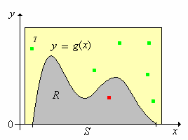
The point of the theorem is that if we can simulate a sequence of independent variables that are uniformly distributed on \( T \), then we can simulate a random variable with the given probability density function \( g \). Suppose in particular that \( R \) is bounded as a subset of \( \R^{n+1} \), which would mean that the domain \( S \) is bounded as a subset of \( \R^n \) and that the probability density function \( g \) is bounded on \( S \). In this case, we can find \( T \) that is the Cartesian product of \( n + 1 \) bounded intervals with \( R \subseteq T \). It turns out to be very easy to simulate a sequence of independent variables, each uniformly distributed on such a product set, so the rejection method always works in this case. As you might guess, the rejection method works best if the size of \( T \), namely \( \lambda_{n+1}(T) \), is small, so that the success parameter \( p \) is large.
The rejection method app simulates a number of continuous distributions via the rejection method. For each of the following distributions, vary the parameters and note the shape and location of the probability density function. Then run the experiment 1000 times and observe the results.
Suppose that a population consists of \(m\) objects, and that each object is one of four types. There are \(a\) type 1 objects, \(b\) type 2 objects, \(c\) type 3 objects and \(m - a - b - c\) type 0 objects. We sample \(n\) objects from the population at random, and without replacement. The parameters \(m\), \(a\), \(b\), \(c\), and \(n\) are nonnegative integers with \(a + b + c \le m\) and \(n \le m\). Denote the number of type 1, 2, and 3 objects in the sample by \(X\), \(Y\), and \(Z\), respectively. Hence, the number of type 0 objects in the sample is \(n - X - Y - Z\). In the problems below, the variables \(x\), \(y\), and \(z\) take values in \(\N\).
\((X, Y, Z)\) has a (multivariate) hypergeometric distribution with probability density function \(f\) given by \[f(x, y, z) = \frac{\binom{a}{x} \binom{b}{y} \binom{c}{z} \binom{m - a - b - c}{n - x - y - z}}{\binom{m}{n}}, \quad x + y + z \le n\]
From basic combinatorics, the numerator is the number of ways to select an unordered sample of size \( n \) from the population with \( x \) objects of type 1, \( y \) objects of type 2, \( z \) objects of type 3, and \( n - x - y - z \) objects of type 0. The denominator is the total number of ways to select the unordered sample.
\((X, Y)\) also has a (multivariate) hypergeometric distribution, with the probability density function \(g\) given by \[g(x, y) = \frac{\binom{a}{x} \binom{b}{y} \binom{m - a - b}{n - x - y}}{\binom{m}{n}}, \quad x + y \le n\]
This result could be obtained by summing the joint density function in over \( z \) for fixed \( (x, y) \). However, there is a much nicer combinatorial argument. Note that we are selecting a random sample of size \(n\) from a population of \(m\) objects, with \(a\) objects of type 1, \(b\) objects of type 2, and \(m - a - b\) objects of other types.
\(X\) has an ordinary hypergeometric distribution, with probability density function \(h\) given by \[h(x) = \frac{\binom{a}{x} \binom{m - a}{n - x}}{\binom{m}{n}}, \quad x \le n\]
Again, the result could be obtained by summing the joint density function in for \( (X, Y, Z) \) over \( (y, z) \) for fixed \( x \), or by summing the joint density function in for \( (X, Y) \) over \( y \) for fixed \( x \). But as before, there is a much more elegant combinatorial argument. Note that we are selecting a random sample of size \(n\) from a population of size \(m\) objects, with \(a\) objects of type 1 and \(m - a\) objects of other types.
These results generalize in a straightforward way to a population with any number of types. In brief, if a random vector has a hypergeometric distribution, then any sub-vector also has a hypergeometric distribution. In other words, all of the marginal distributions of a hypergeometric distribution are themselves hypergeometric. Note however, that it's not a good idea to memorize the formulas above explicitly. It's better to just note the patterns and recall the combinatorial meaning of the binomial coefficient. The hypergeometric distribution and the multivariate hypergeometric distribution are studied in more detail in the chapter on finite sampling models.
Suppose that a population of voters consists of 50 democrats, 40 republicans, and 30 independents. A sample of 10 voters is chosen at random from the population (without replacement, of course). Let \(X\) denote the number of democrats in the sample and \(Y\) the number of republicans in the sample. Find the probability density function of each of the following:
In the formulas for the density functions below, the variables \(x\) and \(y\) are nonnegative integers.
Suppose that the Math Club at Enormous State University (ESU) has 50 freshmen, 40 sophomores, 30 juniors and 20 seniors. A sample of 10 club members is chosen at random to serve on the \(\pi\)-day committee. Let \(X\) denote the number freshmen on the committee, \(Y\) the number of sophomores, and \(Z\) the number of juniors.
In the formulas for the density functions below, the variables \(x\), \(y\), and \(z\) are nonnegative integers.
Suppose that we have a sequence of \(n\) independent trials, each with 4 possible outcomes. On each trial, outcome 1 occurs with probability \(p\), outcome 2 with probability \(q\), outcome 3 with probability \(r\), and outcome 0 occurs with probability \(1 - p - q - r\). The parameters \(p\), \(q\), and \(r\) are nonnegative numbers with \(p + q + r \le 1\), and \(n \in \N_+\). Denote the number of times that outcome 1, outcome 2, and outcome 3 occurred in the \(n\) trials by \(X\), \(Y\), and \(Z\) respectively. Of course, the number of times that outcome 0 occurs is \(n - X - Y - Z\). In the problems below, the variables \(x\), \(y\), and \(z\) take values in \(\N\).
\((X, Y, Z)\) has a multinomial distribution with probability density function \(f\) given by \[f(x, y, z) = \binom{n}{x, \, y, \, z} p^x q^y r^z (1 - p - q - r)^{n - x - y - z}, \quad x + y + z \le n\]
The multinomial coefficient is the number of sequences of length \( n \) with 1 occurring \( x \) times, 2 occurring \( y \) times, 3 occurring \( z \) times, and 0 occurring \( n - x - y - z \) times. The result then follows by independence.
\((X, Y)\) also has a multinomial distribution with the probability density function \(g\) given by \[g(x, y) = \binom{n}{x, \, y} p^x q^y (1 - p - q)^{n - x - y}, \quad x + y \le n\]
This result could be obtained from the joint density function in above, by summing over \( z \) for fixed \( (x, y) \). However there is a much better direct argument. Note that we have \(n\) independent trials, and on each trial, outcome 1 occurs with probability \(p\), outcome 2 with probability \(q\), and some other outcome with probability \(1 - p - q\).
\(X\) has a binomial distribution, with the probability density function \(h\) given by \[h(x) = \binom{n}{x} p^x (1 - p)^{n - x}, \quad x \le n\]
Again, the result could be obtained by summing the joint density function in for \( (X, Y, Z) \) over \( (y, z) \) for fixed \( x \) or by summing the joint density function in for \( (X, Y) \) over \( y \) for fixed \( x \). But as before, there is a much better direct argument. Note that we have \(n\) independent trials, and on each trial, outcome 1 occurs with probability \(p\) and some other outcome with probability \(1 - p\).
These results generalize in a completely straightforward way to multinomial trials with any number of trial outcomes. In brief, if a random vector has a multinomial distribution, then any sub-vector also has a multinomial distribution. In other terms, all of the marginal distributions of a multinomial distribution are themselves multinomial. The binomial distribution and the multinomial distribution are studied in more detail in chapter on Bernoulli trials.
Suppose that a system consists of 10 components that operate independently. Each component is working with probability \(\frac{1}{2}\), idle with probability \(\frac{1}{3}\), or failed with probability \(\frac{1}{6}\). Let \(X\) denote the number of working components and \(Y\) the number of idle components. Give the probability density function of each of the following:
In the formulas below, the variables \(x\) and \(y\) are nonnegative integers.
Suppose that in a crooked, four-sided die, face \(i\) occurs with probability \(\frac{i}{10}\) for \(i \in \{1, 2, 3, 4\}\). The die is thrown 12 times; let \(X\) denote the number of times that score 1 occurs, \(Y\) the number of times that score 2 occurs, and \(Z\) the number of times that score 3 occurs.
In the formulas for the density functions below, the variables \(x\), \(y\) and \(z\) are nonnegative integers.
Suppose that \((X, Y)\) has probability the density function \(f\) given below: \[f(x, y) = \frac{1}{12 \pi} \exp\left[-\left(\frac{x^2}{8} + \frac{y^2}{18}\right)\right], \quad (x, y) \in \R^2\]
Suppose that \((X, Y)\) has probability density function \(f\) given below:
\[f(x, y) = \frac{1}{\sqrt{3} \pi} \exp\left[-\frac{2}{3}\left(x^2 - x y + y^2\right)\right], \quad(x, y) \in \R^2\]The joint distributions in the last two exercises are examples of bivariate normal distributions. Normal distributions are widely used to model physical measurements subject to small, random errors. In both exercises, the marginal distributions of \( X \) and \( Y \) also have normal distributions, and this turns out to be true in general.
Recall that the exponential distribution has probability density function \[f(x) = r e^{-r t}, \quad x \in [0, \infty)\] where \(r \in (0, \infty)\) is the rate parameter. The exponential distribution is widely used to model random times, particularly in the context of the Poisson model.
If \(X\) and \(Y\) have exponential distributions with parameters \(a, \, b \in (0, \infty)\) respectively, and are independent, then \(\P(X \lt Y) = \frac{a}{a + b}\).
If \(X\), \(Y\), and \(Z\) have exponential distributions with parameters \(a, \, b, \, c \in (0, \infty)\) respectively, and are independent, then
If \(X\), \(Y\), and \(Z\) are the lifetimes of devices that act independently, then the results in the previous two exercises give probabilities of various failure orders. Results of this type are also very important in the study of continuous-time Markov processes. We will continue this discussion in the section on transformations of random variables.
Suppose \(X\) takes values in the finite set \(\{1, 2, 3\}\), \(Y\) takes values in the interval \([0, 3]\), and that \((X, Y)\) has probability density function \(f\) given by \[f(x, y) = \begin{cases} \frac{1}{3}, & \quad x = 1, \; 0 \le y \le 1 \\ \frac{1}{6}, & \quad x = 2, \; 0 \le y \le 2 \\ \frac{1}{9}, & \quad x = 3, \; 0 \le y \le 3 \end{cases}\]
Suppose that \(P\) takes values in the interval \([0, 1]\), \(X\) takes values in the finite set \(\{0, 1, 2, 3\}\), and that \((P, X)\) has probability density function \(f\) given by \[f(p, x) = 6 \binom{3}{x} p^{x + 1} (1 - p)^{4 - x}, \quad (p, x) \in [0, 1] \times \{0, 1, 2, 3\}\]
As we will see in the section on conditional distributions, the distribution in models the following experiment: a random probability \(P\) is selected, and then a coin with this probability of heads is tossed 3 times; \(X\) is the number of heads. Note that \( P \) has a beta distribution.
Recall that the Bernoulli distribution with parameter \(p \in [0, 1]\) has probability density function \(g\) given by \(g(x) = p^x (1 - p)^{1 - x}\) for \(x \in \{0, 1\}\). Let \(\bs X = (X_1, X_2, \ldots, X_n)\) be a random sample of size \(n \in \N_+\) from the distribution. Give the probability density funcion of \(\bs X\) in simplified form.
\(\bs X\) has density function \(f\) given by \(f(x_1, x_2, \ldots, x_n) = p^y (1 - p)^{n-y}\) for \((x_1, x_2, \ldots, x_n) \in \{0, 1\}^n\), where \(y = x_1 + x_2 + \cdots + x_n\)
The Bernoulli distribution is name for Jacob Bernoulli, and governs an indicator random varible. Hence if \(\bs X\) is a random sample of size \(n\) from the distribution then \(\bs X\) is a sequence of \(n\) Bernoulli trials.
Recall that the geometric distribution on \(\N_+\) with parameter \(p \in (0, 1)\) has probability density function \(g\) given by \(g(x) = p (1 - p)^{x - 1}\) for \(x \in \N_+\). Let \(\bs X = (X_1, X_2, \ldots, X_n)\) be a random sample of size \(n \in \N_+\) from the distribution. Give the probability density function of \(\bs X\) in simplified form.
\(\bs X\) has pdf \(f\) given by \(f(x_1, x_2, \ldots, x_n) = p^n (1 - p)^{y-n}\) for \((x_1, x_2, \ldots, x_n) \in \N_+^n\), where \(y = x_1 + x_2 + \cdots + x_n\).
The geometric distribution governs the trial number of the first success in a sequence of Bernoulli trials. Hence the variables in the random sample can be interpreted as the number of trials between successive successes.
Recall that the Poisson distribution with parameter \(a \in (0, \infty)\) has probability density function \(g\) given by \(g(x) = e^{-a} \frac{a^x}{x!}\) for \(x \in \N\). Let \(\bs X = (X_1, X_2, \ldots, X_n)\) be a random sample of size \(n \in \N_+\) from the distribution. Give the probability density funcion of \(\bs X\) in simplified form.
\(\bs X\) has density function \(f\) given by \(f(x_1, x_2, \ldots, x_n) = \frac{1}{x_1! x_2! \cdots x_n!} e^{-n a} a^y\) for \((x_1, x_2, \ldots, x_n) \in \N^n\), where \(y = x_1 + x_2 + \cdots + x_n\).
The Poisson distribution is named for Simeon Poisson, and governs the number of random points in a region of time or space under appropriate circumstances. The parameter \( a \) is proportional to the size of the region.
Recall again that the exponential distribution with rate parameter \(r \in (0, \infty)\) has probability density function \(g\) given by \(g(x) = r e^{-r x}\) for \(x \in (0, \infty)\). Let \(\bs X = (X_1, X_2, \ldots, X_n)\) be a random sample of size \(n \in \N_+\) from the distribution. Give the probability density funcion of \(\bs X\) in simplified form.
\(\bs X\) has density function \(f\) given by \(f(x_1, x_2, \ldots, x_n) = r^n e^{-r y}\) for \((x_1, x_2, \ldots, x_n) \in [0, \infty)^n\), where \(y = x_1 + x_2 + \cdots + x_n\).
The exponential distribution governs failure times and other types or arrival times under appropriate circumstances. The variables in the random sample can be interpreted as the times between successive arrivals in the Poisson process.
Recall that the standard normal distribution has probability density function \(\phi\) given by \(\phi(z) = \frac{1}{\sqrt{2 \pi}} e^{-z^2 / 2}\) for \(z \in \R\). Let \(\bs Z = (Z_1, Z_2, \ldots, Z_n)\) be a random sample of size \(n \in \N_+\) from the distribution. Give the probability density funcion of \(\bs Z\) in simplified form.
\(\bs Z\) has density function \(f\) given by \(f(z_1, z_2, \ldots, z_n) = \frac{1}{(2 \pi)^{n/2}} e^{-\frac{1}{2} w^2}\) for \((z_1, z_2, \ldots, z_n) \in \R^n\), where \(w^2 = z_1^2 + z_2^2 + \cdots + z_n^2\).
The standard normal distribution governs physical quantities, properly scaled and centered, subject to small, random errors.
For the cicada data, \(G\) denotes gender and \(S\) denotes species type.
The empirical joint and marginal empirical densities are given in the table below. Gender and species are probably dependent (compare the joint density with the product of the marginal densities).
| \(f(i, j)\) | \(i = 0\) | 1 | \(h(j)\) |
|---|---|---|---|
| \(j = 0\) | \(\frac{16}{104}\) | \(\frac{28}{104}\) | \(\frac{44}{104}\) |
| 1 | \(\frac{3}{104}\) | \(\frac{3}{104}\) | \(\frac{6}{104}\) |
| 2 | \(\frac{40}{104}\) | \(\frac{14}{104}\) | \(\frac{56}{104}\) |
| \(g(i)\) | \(\frac{59}{104}\) | \(\frac{45}{104}\) | 1 |
For the cicada data, let \(W\) denote body weight (in grams) and \(L\) body length (in millimeters).
The empirical joint and marginal densities, based on simple partitions of the body weight and body length ranges, are given in the table below. Body weight and body length are almost certainly dependent.
| Density \((W, L)\) | \(w \in (0, 0.1]\) | \((0.1, 0.2]\) | \((0.2, 0.3]\) | \((0.3, 0.4]\) | Density \(L\) |
|---|---|---|---|---|---|
| \(l \in (15, 20]\) | 0 | 0.0385 | 0.0192 | 0 | 0.0058 |
| \((20, 25]\) | 0.1731 | 0.9808 | 0.4231 | 0 | 0.1577 |
| \((25, 30]\) | 0 | 0.1538 | 0.1731 | 0.0192 | 0.0346 |
| \((30, 35]\) | 0 | 0 | 0 | 0.0192 | 0.0019 |
| Density \(W\) | 0.8654 | 5.8654 | 3.0769 | 0.1923 |
For the cicada data, let \(G\) denote gender and \(W\) body weight (in grams).
The empirical joint and marginal densities, based on a simple partition of the body weight range, are given in the table below. Body weight and gender are almost certainly dependent.
| Density \((W, G)\) | \(w \in (0, 0.1]\) | \((0.1, 0.2]\) | \((0.2, 0.3]\) | \((0.3, 0.4]\) | Density \(G\) |
|---|---|---|---|---|---|
| \(g = 0\) | 0.1923 | 2.5000 | 2.8846 | 0.0962 | 0.5673 |
| 1 | 0.6731 | 3.3654 | 0.1923 | 0.0962 | 0.4327 |
| Density \(W\) | 0.8654 | 5.8654 | 3.0769 | 0.1923 |