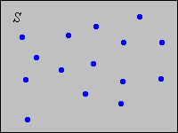
Our starting point in this section is a discrete space \((S, \ms S)\), so that \(S\) is a countable set and \(\ms S\) is the collection of all subsets of \(S\). Counting measure \(\#\) is the standard reference measure for \((S, \ms S)\) so \(\#(A)\) is simply the number of elements in \(A\) for \(A \in \ms S\). If \(P\) is a probability measure on \((S, \ms S)\) then \((S, \ms S, P)\) is a discrete probability space, the simplest kind and the subject of this section. In the picture below, the blue dots are intended to represent points of positive probability.
Most of the results in the basic theory that follows are special cases of general results given in the introduction. But we give independent proofs because they are so simple and can give insight, particularly to a new student of probability. First it's very simple to describe a discrete probability distribution with the function that assigns probabilities to the individual points in \(S\).
Suppose that \(P\) is a probability measure on \((S, \ms S)\). The function \(f\) on \(S\) defined by \( f(x) = P(\{x\}) \) for \( x \in S \) is the probability density function of \(P\), and satisfies the folloing properties:
These properties follow from the axioms of a probability measure.
Part (c) of means that \(f\) really is the density function of \(P\) relative to \(\#\), and is particularly important since it means that a discrete probability distribution is completely determined by its probability density function. Conversely, any function that satisfies properties (a) and (b) of can be used to construct a discrete probability distribution on \(S\) via property (c).
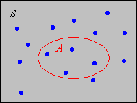
A nonnegative function \(f\) on \(S\) that satisfies \(\sum_{x \in S} f(x) = 1\) is a probability density function, and then \(P\) defined below is a probability measure on \((S, \ms S)\). \[P(A) = \sum_{x \in A} f(x), \quad A \in \ms S\]
Once again, \(f\) is the density of \(P\) relative to \(\#\).
The set \(S\) is often a countable subset of some larger set, such as \(\R^n\) for some \(n \in \N_+\). But not always. We might want to consider a random variable with values in a deck of cards, or a set of words, or some other discrete population of objects. Of course, we can always map a countable set \( S \) one-to-one into a Euclidean set, but it might be contrived or unnatural to do so. In any event, if \( S \) is a subset of a larger set, we can always extend a probability density function \(f\), if we want, to the larger set by defining \(f(x) = 0\) for \(x \notin S\). Sometimes this extension simplifies formulas and notation. Put another way, the set \(S\) is often a convenience set that includes the points with positive probability, but perhaps other points as well.
Suppose that \(f\) is a probability density function on \(S\). Then \(\{x \in S: f(x) \gt 0\}\) is the support set of the distribution.
Values of \( x \) that maximize the probability density function are important enough to deserve a name.
Suppose again that \(f\) is a probability density function on \(S\). An element \(x \in S\) that maximizes \(f\) is a mode of the distribution.
When there is only one mode, it is sometimes used as a measure of the center of the distribution.
A discrete probability distribution defined by a probability density function \(f\) is equivalent to a discrete mass distribution, with total mass 1. In this analogy, \(S\) is the (countable) set of point masses, and \(f(x)\) is the mass of the point at \(x \in S\). Property (c) in simply means that the mass of a set \(A\) can be found by adding the masses of the points in \(A\). But let's consider a probabilistic interpretation, rather than one from physics.
Suppose that \(X\) is a random variable for an experiment and that \(X\) has a discrete distribution on \(S\) with probability density function \(f\). The experiment is repeated independently to produce a sequence \(\bs{X} = (X_1, X_2, \ldots)\) of independent copies of \(X\). For \(n \in \N_+\) define \[f_n(x) = \frac{1}{n} \#\left\{ i \in \{1, 2, \ldots, n\}: X_i = x\right\} = \frac{1}{n} \sum_{i=1}^n \bs{1}(X_i = x), \quad x \in S\] so that \(f_n(x)\) is the relative frequency of outcome \(x \in S\) in the first \(n\) runs. The function \(f_n\) is called the empirical probability density function based on the first \(n\) runs.
In statistical terms, \(\bs{X}\) is produced by sampling from the distribution of \(X\). Note also that \(f_n(x)\) is a random variable for the compound experiment for each \(x \in S\), and in fact \(f_n\) a (random) probability density function, since it satisfies the defining properties in .
By the law of large numbers, \(f_n(x)\) converge sto \(f(x)\) as \(n \to \infty\).
Empirical density functions are displayed in most of the simulation apps that deal with discrete variables, so you will be able to see the law of large numbers at work. It's easy to construct discrete probability density functions from other nonnegative functions defined on a countable set.
Suppose that \(g\) is a nonnegative function defined on \(S\), and let \[c = \sum_{x \in S} g(x)\] If \(0 \lt c \lt \infty\), then the function \(f\) defined by \(f(x) = \frac{1}{c} g(x)\) for \(x \in S\) is a probability density function on \(S\).
Note that since we are assuming that \(g\) is nonnegative, \(c = 0\) if and only if \(g(x) = 0\) for every \(x \in S\). At the other extreme, \(c = \infty\) could only occur if \(S\) is infinite (and the infinite series diverges). When \(0 \lt c \lt \infty\) (so that we can construct the probability density function \(f\)), \(c\) is sometimes called the normalizing constant. This result is useful for constructing probability density functions with desired functional properties (domain, shape, symmetry, and so on).
Suppose again that \(X\) is a random variable on a probability space \((\Omega, \ms F, \P)\) and that \(X\) takes values in our discrete set \(S\). The distributionn of \(X\) (and hence the probability density function of \(X\)) is based on the underlying probability measure on the sample space \((\Omega, \ms F)\). This measure could be a conditional probability measure, conditioned on a given event \(E \in \ms F\) (with \(\P(E) \gt 0\)). The probability density function in this case is \[f(x \mid E) = \P(X = x \mid E), \quad x \in S\] Except for notation, no new concepts are involved. Therefore, all results that hold for discrete probability density functions in general have analogies for conditional discrete probability density functions.
For fixed \(E \in \ms F\) with \(\P(E) \gt 0\) the function \(x \mapsto f(x \mid E)\) is a probability density function on \(S\) That is,
This is a consequence of the fact that \( A \mapsto \P(A \mid E) \) is a probability measure on \((\Omega, \ms F)\). The function \( x \mapsto f(x \mid E) \) is the probability density function of the conditional distribution just as \( f \) is the probability density function of the original distribution.
In particular, the event \( E \) could be an event defined in terms of the random variable \( X \) itself.
Suppose that \(B \subseteq S\) and \(\P(X \in B) \gt 0\). The conditional probability density function of \(X\) given \(X \in B\) is the function on \(B\) defined by \[f(x \mid X \in B) = \frac{f(x)}{\P(X \in B)} = \frac{f(x)}{\sum_{y \in B} f(y)}, \quad x \in B \]
Note that the denominator is simply the normalizing constant in for \( f \) restricted to \( B \). Of course, \(f(x \mid B) = 0\) for \(x \in B^c\).
Suppose again that \(X\) is a random variable defined on a probability space \((\Omega, \ms F, \P)\) and that \(X\) has a discrete distribution on \(S\), with probability density function \(f\). We assume that \( f(x) \gt 0 \) for \( x \in S \) so that the distribution has support \(S\). The versions of the law of total probability in and Bayes' theorem in follow immediately from the corresponding results in the section on conditional probabiity. Only the notation is different.
Law of Total Probability. If \(E \in \ms F\) is an event then \[\P(E) = \sum_{x \in S} f(x) \P(E \mid X = x)\]
Note that \(\{\{X = x\}: x \in S\}\) is a countable partition of the sample set \(\Omega\). That is, these events are disjoint and their union is \(\Omega\). Hence \[ \P(E) = \sum_{x \in S} \P(E \cap \{X = x\}) = \sum_{x \in S} \P(X = x) \P(E \mid X = x) = \sum_{x \in S} f(x) \P(E \mid X = x) \]
This result is useful, naturally, when the distribution of \(X\) and the conditional probability of \(E\) given the values of \(X\) are known. When we compute \(\P(E)\) in this way, we say that we are conditioning on \(X\). Note that \( \P(E) \), as expressed by the formula, is a weighted average of \( \P(E \mid X = x) \), with weight factors \( f(x) \), over \( x \in S \).
Bayes' Theorem. If \(E \in \ms F\) is an event with \(\P(E) \gt 0\) then \[f(x \mid E) = \frac{f(x) \P(E \mid X = x)}{\sum_{y \in S} f(y) \P(E \mid X = y)}, \quad x \in S\]
Bayes' theorem, named for Thomas Bayes, is a formula for the conditional probability density function of \(X\) given \(E\). Again, it is useful when the quantities on the right are known. In the context of Bayes' theorem, the (unconditional) distribution of \(X\) is referred to as the prior distribution and the conditional distribution as the posterior distribution. Note that the denominator in Bayes' formula is \(\P(E)\) and is simply the normalizing constant as in for the function \(x \mapsto f(x) \P(E \mid X = x)\).
We start with some simple (albeit somewhat artificial) discrete distributions. After that, we study three special parametric models—the discrete uniform distribution, hypergeometric distributions, and Bernoulli trials. These models are very important, so when working the computational problems that follow, try to see if the problem fits one of these models. As always, be sure to try the problems yourself before looking at the answers and proofs in the text.
Let \(g\) be the function defined by \(g(n) = n (10 - n)\) for \(n \in \{1, 2, \ldots, 9\}\).
Let \(g\) be the function defined by \(g(n) = n^2 (10 -n)\) for \(n \in \{1, 2 \ldots, 10\}\).
Let \(g\) be the function defined by \(g(x, y) = x + y\) for \((x, y) \in \{1, 2, 3\}^2\).
Let \(g\) be the function defined by \(g(x, y) = x y\) for \((x, y) \in \{(1, 1), (1,2), (1, 3), (2, 2), (2, 3), (3, 3)\}\).
Consider the following game: An urn initially contains one red and one green ball. A ball is selected at random, and if the ball is green, the game is over. If the ball is red, the ball is returned to the urn, another red ball is added, and the game continues. At each stage, a ball is selected at random, and if the ball is green, the game is over. If the ball is red, the ball is returned to the urn, another red ball is added, and the game continues. Let \( X \) denote the length of the game (that is, the number of selections required to obtain a green ball). Find the probability density function of \( X \).
Note that \(X\) takes values in \(\N_+\). Using the multiplication rule for conditional probabilities, the probability density function \(f\) of \(X\) is given by \[f(1) = \frac{1}{2} = \frac{1}{1 \cdot 2}, \; f(2) = \frac{1}{2} \frac{1}{3} = \frac{1}{2 \cdot 3}, \; f(3) = \frac{1}{2} \frac{2}{3} \frac{1}{4} = \frac{1}{3 \cdot 4}\] and in general, \(f(x) = \frac{1}{x (x + 1)}\) for \(x \in \N_+\). By partial fractions, \(f(x) = \frac{1}{x} - \frac{1}{x + 1}\) for \(x \in \N_+\) so we can check that \(f\) is a valid PDF: \[\sum_{x=1}^\infty \left(\frac{1}{x} - \frac{1}{x+1}\right) = \lim_{n \to \infty} \sum_{x=1}^n \left(\frac{1}{x} - \frac{1}{x+1}\right) = \lim_{n \to \infty} \left(1 - \frac{1}{n+1}\right) = 1\]
An element \(X\) is chosen at random from a finite set \(S\). The distribution of \(X\) is the discrete uniform distribution on \(S\).
The phrase at random means that all outcomes are equally likely.
Many random variables that arise in sampling or combinatorial experiments are transformations of uniformly distributed variables. The next few exercises review the standard methods of sampling from a finite population. The parameters \(m\) and \(n\) are positive inteters.
Suppose that \(n\) elements are chosen at random, with replacement from a set \(D\) with \(m\) elements. Let \(\bs{X}\) denote the ordered sequence of elements chosen. Then \(\bs X\) is uniformly distributed on the Cartesian power set \(S = D^n\), and has probability density function \(f\) given by \[f(\bs{x}) = \frac{1}{m^n}, \quad \bs{x} \in S\]
Recall that \( \#(D^n) = m^n \).
Suppose that \(n\) elements are chosen at random, without replacement from a set \(D\) with \(m\) elements (so \(n \le m\)). Let \(\bs{X}\) denote the ordered sequence of elements chosen. Then \(\bs X\) is uniformly distributed on the set \(S\) of permutations of size \(n\) chosen from \(D\), and has probability density function \(f\) given by \[f(\bs{x}) = \frac{1}{m^{(n)}}, \quad \bs{x} \in S\]
Recall that the number of permutations of size \( n \) from \( D \) is \( m^{(n)} \).
Suppose that \(n\) elements are chosen at random, without replacement, from a set \(D\) with \(m\) elements (so \(n \le m\)). Let \(\bs Y\) denote the unordered set of elements chosen. Then \(\bs Y\) is uniformly distributed on the set \(T\) of combinations of size \(n\) chosen from \(D\), and has probability density function \(f\) given by \[f(\bs y) = \frac{1}{\binom{m}{n}}, \quad \bs y\in T\]
Recall that the number of combinations of size \( n \) from \( D \) is \( \binom{m}{n} \).
Suppose that \(X\) is uniformly distributed on a finite set \(S\) and that \(B\) is a nonempty subset of \(S\). Then the conditional distribution of \(X\) given \(X \in B\) is uniform on \(B\).
Recall that a dichotomous population consists of \(m \in \N_+\) objects of two different types: \(r\) of the objects are type 1 and \(m - r\) are type 0, where \(r \in \{0, 1, \ldots, m\}\). Here are some typical examples:
A sample of \(n\) objects is chosen at random (without replacement) from the population, so that \(n \in \{0, 1, \ldots, m\}\).
Recall again that the phrase at random means that the samples, either ordered or unordered are equally likely. Note that this probability model has three parameters: the population size \(m\), the number of type 1 objects \(r\), and the sample size \(n\). Now, suppose that we keep track of order, and let \(X_i\) denote the type of the \(i\)th object chosen, for \(i \in \{1, 2, \ldots, n\}\). Thus, \(X_i\) is an indicator variable (that is, a variable that just takes values 0 and 1).
\(\bs{X} = (X_1, X_2, \ldots, X_n) \) has probability density function \( f \) given by \[ f(x_1, x_2, \ldots, x_n) = \frac{r^{(y)} (m - r)^{(n - y)}}{m^{(n)}}, \quad (x_1, x_2, \ldots, x_n) \in \{0, 1\}^n \text{ where } y = x_1 + x_2 + \cdots + x_n \]
Recall again that the ordered samples are equally likely, and there are \( m^{(n)} \) such samples. The number of ways to select the \( y \) type 1 objects and place them in the positions where \( x_i = 1 \) is \( r^{(y)} \). The number of ways to select the \( n - y \) type 0 objects and place them in the positions where \( x_i = 0 \) is \( (m - r)^{(n - y)} \). Thus the result follows from the multiplication principle.
Note that the value of \( f(x_1, x_2, \ldots, x_n) \) depends only on \( y = x_1 + x_2 + \cdots + x_n \), and hence is unchanged if \( (x_1, x_2, \ldots, x_n) \) is permuted. This means that \((X_1, X_2, \ldots, X_n) \) is exchangeable. In particular, the distribution of \( X_i \) is the same as the distribution of \( X_1 \), so \[ \P(X_i = 1) = \frac{r}{m} \] Thus, the variables are identically distributed. Also the distribution of \( (X_i, X_j) \) is the same as the distribution of \( (X_1, X_2) \), so \[ \P(X_i = 1, X_j = 1) = \frac{r (r - 1)}{m (m - 1)} \] Thus, \( X_i \) and \( X_j \) are not independent, and in fact are negatively correlated. Now let \(Y\) denote the number of type 1 objects in the sample. Note that \(Y = \sum_{i = 1}^n X_i\). Any counting variable can be written as a sum of indicator variables.
\(Y\) has probability density function \( g \) given by. \[g(y) = \frac{\binom{r}{y} \binom{m - r}{n - y}}{\binom{m}{n}}, \quad y \in \{0, 1, \ldots, n\}\]
Recall again that the unordered samples of size \( n \) chosen from the population are equally likely. By the multiplication principle, the number of samples with exactly \( y \) type 1 objects and \( n - y \) type 0 objects is \( \binom{m}{y} \binom{m - r}{n - y} \). The total number of samples is \( \binom{m}{n} \).
The distribution defined in is the hypergeometric distributions with parameters \(m\), \(r\), and \(n\). The term hypergeometric comes from a certain class of special functions, but is not particularly helpful in terms of remembering the model. Nonetheless, we are stuck with it. The set of values \( \{0, 1, \ldots, n\} \) is a convenience set: it contains all of the values that have positive probability, but depending on the parameters, some of the values may have probability 0. Recall our convention for binomial coefficients: for \( j, \; k \in \N_+ \), \( \binom{k}{j} = 0 \) if \( j \gt k \). Note also that the hypergeometric distribution is unimodal: the probability density function increases and then decreases, with either a single mode or two adjacent modes. We can extend the hypergeometric model to a population of three types.
Consider a trichotomous population consists of \(m \in \N_+\) objects; \(r\) of the objects are type 1, \(s\) are type 2, and \(m - r - s\) are type 0, where \(r, \, s \in \N_+\) with \(r + s \le m\). Here are some examples:
Once again, a sample of \(n\) objects is chosen at random (without replacement) from the population, so \(n \in \{0, 1, \ldots, m\}\).
The probability model now has four parameters: the population size \(m\), the type sizes \(r\) and \(s\), and the sample size \(n\). Moreover, we now need two random variables to keep track of the counts for the three types in the sample. Let \(Y\) denote the number of type 1 objects in the sample and \(Z\) the number of type 2 objects in the sample.
\((Y, Z)\) has probability density function \( h \) given by \[h(y, z) = \frac{\binom{r}{y} \binom{s}{z} \binom{m - r - s}{n - y - z}}{\binom{m}{n}}, \quad (y, z) \in \{0, 1, \ldots, n\}^2 \text{ with } y + z \le n\]
Once again, by the multiplication principle, the number of samples of size \( n \) from the population with exactly \( y \) type 1 objects, \( z \) type 2 objects, and \( n - y - z \) type 0 objects is \( \binom{r}{y} \binom{s}{z} \binom{m - r - s}{n - y - z} \). The total number of samples of size \( n \) is \( \binom{m}{n} \).
The distribution defined in is the bivariate hypergeometric distribution with parameters \(m\), \(r\), \(s\), and \(n\). Once again, the domain given is a convenience set; it includes the set of points with positive probability, but depending on the parameters, may include points with probability 0. Clearly, the same general pattern applies to populations with even more types. However, because of all of the parameters, the formulas are not worthing remembering in detail; rather, just note the pattern, and remember the combinatorial meaning of the binomial coefficient. The hypergeometric model will be revisited later in the sections on joint distributions and conditional distributions. The hypergeometric distribution and the multivariate hypergeometric distribution are studied in detail in the chapter on finite sampling models. This chapter contains a variety of distributions that are based on discrete uniform distributions.
A Bernoulli trials sequence is a sequence \((X_1, X_2, \ldots)\) of independent, identically distributed indicator variables. Random variable \(X_i\) is the outcome of trial \(i\), where in the usual terminology of reliability, 1 denotes success while 0 denotes failure, The process is named for Jacob Bernoulli. Let \(p = \P(X_i = 1) \in [0, 1]\) denote the success parameter of the process. Note that the indicator variables in the hypergeometric model above satisfy one of the assumptions of Bernoulli trials (identical distributions) but not the other (independence).
\(\bs{X} = (X_1, X_2, \ldots, X_n)\) has probability density function \( f \) given by \[f(x_1, x_2, \ldots, x_n) = p^y (1 - p)^{n - y}, \quad (x_1, x_2, \ldots, x_n) \in \{0, 1\}^n, \text{ where } y = x_1 + x_2 + \cdots + x_n\]
By definition, \( \P(X_i = 1) = p \) and \( \P(X_i = 0) = 1 - p \). Equivalently, \( \P(X_i = x) = p^x (1 - p)^{1-x} \) for \( x \in \{0, 1\} \). The formula for \( f \) then follows by independence.
Now let \(Y\) denote the number of successes in the first \(n\) trials. Note that \(Y = \sum_{i=1}^n X_i\), so we see again that a complicated random variable can be written as a sum of simpler ones. In particular, a counting variable can always be written as a sum of indicator variables.
\(Y\) has probability density function \( g \) given by \[g(y) = \binom{n}{y} p^y (1 - p)^{n-y}, \quad y \in \{0, 1, \ldots, n\}\]
From , any particular sequence of \( n \) Bernoulli trials with \( y \) successes and \( n - y \) failures has probability \( p^y (1 - p)^{n - y}\). The number of such sequences is \( \binom{n}{y} \), so the formula for \( g \) follows by the additivity of probability.
The distribution defined in is called the binomial distribution with parameters \(n\) and \(p\). The distribution is unimodal: the probability density function at first increases and then decreases, with either a single mode or two adjacent modes.
Suppose that \(p \gt 0\) and let \(N\) denote the trial number of the first success. Then \(N\) has probability density function \(h\) given by \[h(n) = (1 - p)^{n-1} p, \quad n \in \N_+\] The probability density function \( h \) is decreasing and the mode is \( n = 1 \).
For \( n \in \N_+ \), the event \( \{N = n\} \) means that the first \( n - 1 \) trials were failures and trial \( n \) was a success. Each trial results in failure with probability \( 1 - p \) and success with probability \( p \), and the trials are independent, so \( \P(N = n) = (1 - p)^{n - 1} p \). Using geometric series, we can check that \[\sum_{n=1}^\infty h(n) = \sum_{n=1}^\infty p (1 - p)^{n-1} = \frac{p}{1-(1-p)} = 1\]
The distribution defined in is the geometric distribution on \(\N_+\) with parameter \(p\).
In the following exercises, be sure to check if the problem fits one of the general models above.
An urn contains 30 red and 20 green balls. A sample of 5 balls is selected at random, without replacement. Let \(Y\) denote the number of red balls in the sample.
In the ball and urn experiment, select sampling without replacement and set \(m = 50\), \(r = 30\), and \(n = 5\). Run the experiment 1000 times and compare the empirical density function of \(Y\) with the probability density function.
An urn contains 30 red and 20 green balls. A sample of 5 balls is selected at random, with replacement. Let \(Y\) denote the number of red balls in the sample.
In the ball and urn experiment, select sampling with replacement and set \(m = 50\), \(r = 30\), and \(n = 5\). Run the experiment 1000 times and compare the empirical density function of \(Y\) with the probability density function.
A group of voters consists of 50 democrats, 40 republicans, and 30 independents. A sample of 10 voters is chosen at random, without replacement. Let \(X\) denote the number of democrats in the sample and \(Y\) the number of republicans in the sample.
The Math Club at Enormous State University (ESU) has 20 freshmen, 40 sophomores, 30 juniors, and 10 seniors. A committee of 8 club members is chosen at random, without replacement to organize \(\pi\)-day activities. Let \(X\) denote the number of freshman in the sample, \(Y\) the number of sophomores, and \(Z\) the number of juniors.
Suppose that a coin with probability of heads \(p\) is tossed repeatedly, and the sequence of heads and tails is recorded.
Suppose that a coin with probability of heads \(p = 0.4\) is tossed 5 times. Let \(Y\) denote the number of heads.
In the binomial coin experiment, set \(n = 5\) and \(p = 0.4\). Run the experiment 1000 times and compare the empirical density function of \(Y\) with the probability density function.
Suppose that a coin with probability of heads \(p = 0.2\) is tossed until heads occurs. Let \(N\) denote the number of tosses.
In the negative binomial experiment, set \(k = 1\) and \(p = 0.2\). Run the experiment 1000 times and compare the empirical density function with the probability density function.
Suppose that two fair, standard dice are tossed and the sequence of scores \((X_1, X_2)\) recorded. Let \(Y = X_1 + X_2\) denote the sum of the scores, \(U = \min\{X_1, X_2\}\) the minimum score, and \(V = \max\{X_1, X_2\}\) the maximum score.
We denote the probability density functions by \(f\), \(g\), \(h_1\), \(h_2\), and \(h\) respectively.
Note that \((U, V)\) in could serve as the outcome of the experiment that consists of throwing two standard dice if we did not bother to record order. Note that this random vector does not have a uniform distribution when the dice are fair. The mistaken idea that this vector should have the uniform distribution was the cause of difficulties in the early development of probability.
In the dice experiment, select \(n = 2\) fair dice. Select the following random variables and note the shape and location of the probability density function. Run the experiment 1000 times. For each of the following variables, compare the empirical density function with the probability density function.
In the die-coin experiment, a fair, standard die is rolled and then a fair coin is tossed the number of times showing on the die. Let \(N\) denote the die score and \(Y\) the number of heads.
Run the die-coin experiment 1000 times. For the number of heads, compare the empirical density function with the probability density function.
Suppose that a bag contains 12 coins: 5 are fair, 4 are biased with probability of heads \(\frac{1}{3}\); and 3 are two-headed. A coin is chosen at random from the bag and tossed 5 times. Let \(V\) denote the probability of heads of the selected coin and let \(Y\) denote the number of heads.
Compare the die-coin experiment with the bag of coins experiment . In the first experiment, we toss a coin with a fixed probability of heads a random number of times. In second experiment, we effectively toss a coin with a random probability of heads a fixed number of times. In both cases, we can think of starting with a binomial distribution and randomizing one of the parameters.
In the coin-die experiment, a fair coin is tossed. If the coin lands tails, a fair die is rolled. If the coin lands heads, an ace-six flat die is tossed (faces 1 and 6 have probability \(\frac{1}{4}\) each, while faces 2, 3, 4, 5 have probability \(\frac{1}{8}\) each). Find the probability density function of the die score \(Y\).
\(f(y) = 5/24\) for \( y \in \{1,6\}\), \(f(y) = 7/24\) for \(y \in \{2, 3, 4, 5\}\)
Run the coin-die experiment 1000 times, with the settings in . Compare the empirical density function with the probability density function.
Suppose that a standard die is thrown 10 times. Let \(Y\) denote the number of times an ace or a six occurred. Give the probability density function of \(Y\) and identify the distribution by name and parameter values in each of the following cases:
Suppose that a standard die is thrown until an ace or a six occurs. Let \(N\) denote the number of throws. Give the probability density function of \(N\) and identify the distribution by name and parameter values in each of the following cases:
Fred and Wilma takes turns tossing a coin with probability of heads \(p \in (0, 1)\): Fred first, then Wilma, then Fred again, and so forth. The first person to toss heads wins the game. Let \(N\) denote the number of tosses, and \(W\) the event that Wilma wins.
The random experiment in is known as the alternating coin tossing game.
Suppose that \(k\) players each have a coin with probability of heads \(p\), where \(k \in \{2, 3, \ldots\}\) and where \(p \in (0, 1)\).
The experiment in is known as the odd man out game.
Recall that a poker hand consists of 5 cards chosen at random and without replacement from a standard deck of 52 cards. Let \(X\) denote the number of spades in the hand and \(Y\) the number of hearts in the hand. Give the probability density function of each of the following random variables, and identify the distribution by name:
Recall that a bridge hand consists of 13 cards chosen at random and without replacement from a standard deck of 52 cards. Let \(N\) denote the number of cards in the hand of denomination 10 or higher.
In bridge, the aces, kings, queens, and jacks are referred to as honor cards or high cards. Find the probability that a bridge hand has 2 aces, 3 kings, 1 queen, 1 jack and 6 non-honor cards.
This problem fits the hypergeometric model, with the deck partitioned into 4 aces, 4 kings, 4 queens, 4 jacks, and 36 non-honor cards. The probability of the event is \[\frac{\binom{4}{2} \binom{4}{3} \binom{4}{1} \binom{4}{1} \binom{36}{6}}{\binom{52}{13}} = \frac{747\,952\,128} {635\,013\,559\,600} = 0.00117785\]
In the most common honor card point system, an ace is worth four points, a king three points, a queen two points, and a jack one point. So the hand in exercise has 17 high card points, which would be considered a strong bridge hand. Finding the density function of the high card value of a random bridge hand is computationally messy, but ultimately just relies on hypergeometric probabiliites of the type in the exercise. Complete details on the high card distribution are in the section on bridge.
Open the bridge app and select High-card value in the drop-down box. Note the shape and location of the density function. Run the experiment 1000 times and compare the empirical density function to the probability density function.
However, evaluating the strength of a bridge hand is much more complicated than just computing the honor points. The distribution of the cards by suit is also very important. For example, the strength of a hand with the queen of hearts is diminished if that card is the only heart.
Find the probability that a bridge hand has no spades, 2 hearts, 5 diamonds and 6 clubs.
This problem also fits the hypergeometric model, with the deck partitioned into 13 cards in each of the four suits. The probability of the event is \[\frac{\binom{13}{0} \binom{13}{2} \binom{13}{5} \binom{13}{6}}{\binom{52}{13}} = \frac{172\,262\,376}{635\,013\,559\,600} = 0.000271274\]
In the most common method for assigning distribution points, a void (a suit with no cards in the hand) is worth three points, a singleton (a suit with one card in the hand) is worth two points, and a doubleton (a suit with two cards in the hand) is worth one point. So the hand in exercise has 4 distribution points, which could also consititue a strong hand, particulalry if the contract is in one of the long suits (diamonds or clubs). Like the honor card points, the probability density function of the suit distribution points is messy, but ultimately relies on hypergeometric probabilities of the type in the exercise. Coplete details are in the section on bridge.
Open the bridge app and select Sparse suit value in the drop-down box. Note the shape and location of the density function. Run the experiment 1000 times and compare the empirical density function to the probability density function.
Suppose that in a batch of 500 components, 20 are defective and the rest are good. A sample of 10 components is selected at random and tested. Let \(X\) denote the number of defectives in the sample.
A plant has 3 assembly lines that produce a certain type of component. Line 1 produces 50% of the components and has a defective rate of 4%; line 2 has produces 30% of the components and has a defective rate of 5%; line 3 produces 20% of the components and has a defective rate of 1%. A component is chosen at random from the plant and tested.
Let \(D\) the event that the item is defective, and \(f(\cdot \mid D)\) the probability density function of the line number given \(D\).
Recall that in the standard model of structural reliability, a systems consists of \(n\) components, each of which, independently of the others, is either working for failed. Let \(X_i\) denote the state of component \(i\), where 1 means working and 0 means failed. Thus, the state vector is \(\bs{X} = (X_1, X_2, \ldots, X_n)\). The system as a whole is also either working or failed, depending only on the states of the components. Thus, the state of the system is an indicator random variable \(U = u(\bs{X})\) that depends on the states of the components according to a structure function \(u: \{0,1\}^n \to \{0, 1\}\). In a series system, the system works if and only if every components works. In a parallel system, the system works if and only if at least one component works. In a \(k\) out of \(n\) system, the system works if and only if at least \(k\) of the \(n\) components work.
The reliability of a device is the probability that it is working. Let \(p_i = \P(X_i = 1)\) denote the reliability of component \(i\), so that \(\bs{p} = (p_1, p_2, \ldots, p_n)\) is the vector of component reliabilities. Because of the independence assumption, the system reliability depends only on the component reliabilities, according to a reliability function \(r(\bs{p}) = \P(U = 1)\). Note that when all component reliabilities have the same value \(p\), the states of the components form a sequence of \(n\) Bernoulli trials. In this case, the system reliability is, of course, a function of the common component reliability \(p\).
Suppose that the component reliabilities all have the same value \(p\). Let \(\bs{X}\) denote the state vector and \(Y\) denote the number of working components.
Suppose that we have 4 independent components, with common reliability \(p = 0.8\). Let \(Y\) denote the number of working components.
Suppose that we have 4 independent components, with reliabilities \(p_1 = 0.6\), \(p_2 = 0.7\), \(p_3 = 0.8\), and \(p_4 = 0.9\). Let \(Y\) denote the number of working components.
Suppose that \( a \in (0, \infty) \). Define the function \( f \) on \(\N\) by \[f(n) = e^{-a} \frac{a^n}{n!}, \quad n \in \N\]
The distribution defined in is the Poisson distribution with parameter \(a\), named after Simeon Poisson. Note that like the other named distributions we studied above (hypergeometric and binomial), the Poisson distribution is unimodal: the probability density function at first increases and then decreases, with either a single mode or two adjacent modes. The Poisson distribution is used to model the number of random points
in a region of time or space, under certain ideal conditions. The parameter \(a\) is proportional to the size of the region of time or space.
Suppose that the customers arrive at a service station according to the Poisson model, at an average rate of 4 per hour. Thus, the number of customers \(N\) who arrive in a 2-hour period has the Poisson distribution with parameter 8.
In the Poisson experiment, set \(r = 4\) and \(t = 2\). Run the simulation 1000 times and compare the empirical density function to the probability density function.
Suppose that the number of flaws \(N\) in a piece of fabric of a certain size has the Poisson distribution with parameter 2.5.
Suppose that the number of raisins \(N\) in a piece of cake has the Poisson distribution with parameter 10.
Let \(g\) be the function defined by \(g(n) = \frac{1}{n^2}\) for \(n \in \N_+\).
The distribution defined in is a member of the family of zeta distributions. Zeta distributions are used to model sizes or ranks of certain types of objects.
Let \(f\) be the function defined by \(f(d) = \log(d + 1) - \log(d) = \log\left(1 + \frac{1}{d}\right)\) for \(d \in \{1, 2, \ldots, 9\}\). (The logarithm function is the base 10 common logarithm, not the base \(e\) natural logarithm.)
| \(d\) | 1 | 2 | 3 | 4 | 5 | 6 | 7 | 8 | 9 |
|---|---|---|---|---|---|---|---|---|---|
| \(f(d)\) | 0.3010 | 0.1761 | 0.1249 | 0.0969 | 0.0792 | 0.0669 | 0.0580 | 0.0512 | 0.0458 |
The distribution defined in is known as Benford's law, and is named for the American physicist and engineer Frank Benford. This distribution governs the leading digit in many real sets of data.
In the M&M data, let \(R\) denote the number of red candies and \(N\) the total number of candies. Compute and graph the empirical probability density function of each of the following:
We denote the PDF of \(R\) by \(f\) and the PDF of \(N\) by \(g\)
| \(r\) | 3 | 4 | 5 | 6 | 8 | 9 | 10 | 11 | 12 | 14 | 15 | 20 |
|---|---|---|---|---|---|---|---|---|---|---|---|---|
| \(f(r)\) | \(\frac{1}{30}\) | \(\frac{3}{30}\) | \(\frac{3}{30}\) | \(\frac{2}{30}\) | \(\frac{4}{30}\) | \(\frac{5}{30}\) | \(\frac{2}{30}\) | \(\frac{1}{30}\) | \(\frac{3}{30}\) | \(\frac{3}{30}\) | \(\frac{3}{30}\) | \(\frac{1}{30}\) |
| \(n\) | 50 | 53 | 54 | 55 | 56 | 57 | 58 | 59 | 60 | 61 |
|---|---|---|---|---|---|---|---|---|---|---|
| \(g(n)\) | \(\frac{1}{30}\) | \(\frac{1}{30}\) | \(\frac{1}{30}\) | \(\frac{4}{30}\) | \(\frac{4}{30}\) | \(\frac{3}{30}\) | \(\frac{9}{30}\) | \(\frac{3}{30}\) | \(\frac{2}{30}\) | \(\frac{2}{30}\) |
| \(r\) | 3 | 4 | 6 | 8 | 9 | 11 | 12 | 14 | 15 |
|---|---|---|---|---|---|---|---|---|---|
| \(f(r \mid N \gt 57)\) | \(\frac{1}{16}\) | \(\frac{1}{16}\) | \(\frac{1}{16}\) | \(\frac{3}{16}\) | \(\frac{3}{16}\) | \(\frac{1}{16}\) | \(\frac{1}{16}\) | \(\frac{3}{16}\) | \(\frac{2}{16}\) |
In the Cicada data, let \(G\) denotes gender, \(T\) species type, and \(W\) body weight (in grams). Compute the empirical probability density function of each of the following:
We denote the probability density functions of \(G\), \(T\), and \((G, T)\) by \(g\), \(h\) and \(f\), respectively.