Conditional expected value is much more important than one might at first think. In fact, conditional expected value is at the core of modern probability theory because it provides the basic way of incorporating known information into a probability measure. This section extends our first study of conditional expected value from a more measure-theoretic point of view.
Basic Theory
Definition
As usual, our starting point is a random experiment , as described in random experiment, modeled by a probability space \((\Omega, \mathscr F, \P)\). So \( \Omega \) is the set of outcomes,, \( \mathscr F \) is the \( \sigma \)-algebra of events, and \( \P \) is the probability measure on the sample space \( (\Omega, \mathscr F) \). Previously we studied the conditional expected value of a real-value random variable \(X\) given a random variable \(Y\). The more general approach is to condition on a sub \(\sigma\)-algebra \( \mathscr G \) of \( \mathscr F \).
Before we get to the definition, we need some preliminaries. First, all random variables mentioned are assumed to be real valued. Next the notion of an equivalence relation plays a fundamental role in this section. In particular, recall that random variables \( X_1 \) and \( X_2 \) are equivalent if \( \P(X_1 = X_2) = 1 \). Equivalence really does define an equivalence relation on the collection of random variables defined on the sample space. Moreover, we often regard equivalent random variables as being essentially the same object. More precisely from this point of view, the objects of our study are not individual random variables but rather equivalence classes of random variables under this equivalence relation. Finally, for \( A \in \mathscr F \), recall the notation for the expected value of \( X \) on the event \( A \)
\[ \E(X; A) = \E(X \bs{1}_A)\]
assuming of course that the expected value exists. For the remainder of this subsection, suppose that \( \mathscr G \) is a sub \( \sigma \)-algebra of \( \mathscr F \).
Suppose that \(X\) is a random variable with \( \E(|X|) \lt \infty \). The conditional expected value of \(X\) given \(\mathscr G\) is the random variable \(\E(X \mid \mathscr G)\) defined by the following properties:
\(\E(X \mid \mathscr G)\) is measurable with repsect to \(\mathscr G\).
If \(A \in \mathscr G\) then \(\E[\E(X \mid \mathscr G); A] = \E(X; A)\)
The basic idea is that \( \E(X \mid \mathscr G) \) is the expected value of \( X \) given the information in the \( \sigma \)-algebra \( \mathscr G \). Hopefully this idea will become clearer during our study. The conditions above uniquely define \( \E(X \mid \mathscr G) \) up to equivalence. The proof of this fact is a simple application of the Radon-Nikodym theorem, named for Johann Radon and Otto Nikodym
Suppose again that \(X\) is a random variable with \( \E(|X|) \lt \infty \).
There exists a random variable \( V \) satisfying definition .
If \( V_1 \) and \( V_2 \) satisfy definition , then \( \P(V_1 = V_2) = 1 \) so that \( V_1 \) and \( V_2 \) are equivalent.
Details:
Note that \( \nu(A) = \E(X; A) \) for \( A \in \mathscr G \) defines a (signed) measure on \( \mathscr G \). Moreover, if \( A \in \mathscr G \) and \( \P(A) = 0 \) then \( \nu(A) = 0 \). Hence \( \nu \) is absolutely continuous with respect to the restriction of \( \P \) to \( \mathscr G \). By the Radon-Nikodym theorem, there exists a random variable \( V \) that is measurable with respect to \( \mathscr G \) such that \( \nu(A) = \E(V; A) \) for \( A \in \mathscr G \). That is, \( V \) is the density or derivative of \( \nu \) with respect to \( \P \) on \( \mathscr G \).
This follows from the uniqueness of the Radon-Nikodym derivative, up to equivalence.
The following characterization might seem stronger but in fact in equivalent to the definition.
Suppose again that \(X\) is a random variable with \( \E(|X|) \lt \infty \). Then \( \E(X \mid \mathscr G) \) is characterized by the following properties:
\( \E(X \mid \mathscr G) \) is measurable with respect to \( \mathscr G \)
If \( U \) is measurable with respect to \( \mathscr G \) and \( \E(|U X|) \lt \infty \) then \( \E[U \E(X \mid \mathscr G)] = \E(U X) \).
Details:
We have to show that part (b) in definition is equivalent to part (b) here. First (b) here implies (b) in the definition since \( \bs{1}_A \) is \( \mathscr G \)-measurable if \( A \in \mathscr G \). Conversely suppose that (b) in the definition holds. We will show that (b) here holds by a classical bootstrapping argument.. First \( \E[U \E(X \mid \mathscr G)] = \E(U X) \) if \( U = \bs{1}_A \) for some \( A \in \mathscr G \). Next suppose that \( U \) is a simple random variable that is \( \mathscr G \)-measurable. That is, \( U = \sum_{i \in I} a_i \bs{1}_{A_i} \) where \( I \) is a finite index set, \( a_i \ge 0 \) for \( i \in I \), and \( A_i \in \mathscr G \) for \( i \in I \). then
\[ \E[U \E(X \mid \mathscr G)] = \E\left[\sum_{i \in I} a_i \bs{1}_{A_i} \E(X \mid \mathscr G)\right] = \sum_{i \in I} a_i \E[\bs{1}_{A_i} \E(X \mid \mathscr G)] = \sum_{i \in I} a_i \E(\bs{1}_{A_i} X) = \E\left(\sum_{i \in I} a_i \bs{1}_{A_i} X\right) = \E(U X) \]
Next suppose that \( U \) is nonnegative and \( \mathscr G \)-measurable. Then there exists a sequence of simple \( \mathscr G \)-measurable random variables \( (U_1, U_2, \ldots) \) with \( U_n \uparrow U \) as \( n \to \infty \). Then by the previous step, \( \E[U_n \E(X \mid \mathscr G)] = \E(U_n X) \) for each \( n \). Letting \( n \to \infty \) and using the monotone convergence theorem we have \( \E[U \E(X \mid \mathscr G)] = \E(U X) \). Finally, suppose that \( U \) is a general \( \mathscr G \)-measurable random variable. Then \( U = U^+ - U^- \) where \( U^+ \) and \( U^- \) are the usual positive and negative parts of \( U \). These parts are nonnegative and \( \mathscr G \)-measurable, so by the previous step, \( \E[U^+ \E(X \mid \mathscr G)] = \E(U^+ X) \) and \( \E[U^- \E(X \mid \mathscr G)] = \E(U^- X) \). hence
\[ \E[U \E(X \mid \mathscr G)] = \E[(U^+ - U^-) \E(X \mid \mathscr G)] = \E[U^+ \E(X \mid \mathscr G)] - \E[U^- \E(X \mid \mathscr G)] = \E(U^+ X) - \E(U^- X) = \E(U X) \]
Properties
Our next discussion concerns some fundamental properties of conditional expected value. All equalities and inequalities are understood to hold modulo equivalence, that is, with probability 1. Note also that many of the proofs work by showing that the right hand side satisfies the properties in definition for the conditional expected value on the left side. Once again we assume that \( \mathscr G \) is a sub \( sigma \)-algebra of \( \mathscr F \).
Our first property is a simple consequence of the definition: \( X \) and \( \E(X \mid \mathscr G) \) have the same mean.
Suppose that \(X\) is a random variable with \( \E(|X|) \lt \infty \). Then \( \E[\E(X \mid \mathscr G)] = \E(X) \).
Details:
This follows immediately by letting \( A = \Omega \) in definition .
Theorem can often be used to compute \( \E(X) \), by choosing the \( \sigma \)-algebra \( \mathscr G \) in a clever way. We say that we are computing \( \E(X) \) by conditioning on \( \mathscr G \). Our next properties are fundamental: every version of expected value must satisfy the linearity properties. The first part is the additive property and the second part is the scaling property.
Suppose that \( X \) and \( Y \) are random variables with \( \E(|X|) \lt \infty \) and \( \E(|Y|) \lt \infty \), and that \( c \in \R\). Then
\( \E(c X \mid \mathscr G) = c \E(X \mid \mathscr G) \)
Details:
Note that \( \E(|X + Y|) \le \E(|X|) + \E(|Y|) \lt \infty\) so \( \E(X + Y \mid \mathscr G) \) is defined. We show that \( \E(X \mid \mathscr G) + \E(Y \mid \mathscr G) \) satisfies the conditions in definition for \( \E(X + Y \mid \mathscr G) \). Note first that \( \E(X \mid \mathscr G) + \E(Y \mid \mathscr G) \) is \( \mathscr G \)-measurable since both terms are. If \(A \in \mathscr G \) then
\[ \E\{[\E(X \mid \mathscr G) + \E(Y \mid \mathscr G)]; A\} = \E[\E(X \mid \mathscr G); A] + \E[\E(Y \mid \mathscr G); A] = \E(X; A) + \E(Y; A) = \E[X + Y; A] \]
Note that \( \E(|c X|) = |c| \E(|X|) \lt \infty \) so \( \E(c X \mid \mathscr G) \) is defined. We show that \( c \E(X \mid \mathscr G) \) satisfy the conditions in definition for \( \E(c X \mid \mathscr G) \). Note first that \( c \E(X \mid \mathscr G) \) is \( \mathscr G \)-measurable since the second factor is. If \(A \in \mathscr G \) then
\[ \E[c \E(X \mid \mathscr G); A] = c \E[\E(X \mid \mathscr G); A] = c \E(X; A) = \E(c X; A) \]
The next set of properties are also fundamental to every notion of expected value. The first part is the positive property and the second part is the increasing property.
Suppose again that \( X \) and \( Y \) are random variables with \( \E(|X|) \lt \infty \) and \( \E(|Y|) \lt \infty \).
If \( X \ge 0 \) then \( \E(X \mid \mathscr G) \ge 0 \)
If \( X \le Y \) then \( \E(X \mid \mathscr G) \le \E(Y \mid \mathscr G) \)
Details:
Let \( A = \{\E(X \mid \mathscr G) \lt 0\} \). Note that \(A \in \mathscr G \) and hence \( \E(X; A) = \E[\E(X \mid \mathscr G); A] \). Since \( X \ge 0 \) with probability 1 we have \( E(X; A) \ge 0 \). On the other hand, if \( \P(A) \gt 0 \) then \( \E[\E(X \mid \mathscr G); A] \lt 0 \) which is a contradiction. Hence we must have \( \P(A) = 0 \).
Note that if \( X \le Y \) then \( Y - X \ge 0 \). Hence by (a) and the additive property, \( \E(Y - X \mid \mathscr G) = \E(Y \mid \mathscr G) - \E(X \mid \mathscr G) \ge 0 \) so \( \E(Y \mid \mathscr G) \ge \E(X \mid \mathscr G) \).
The next few properties relate to the central idea that \( \E(X \mid \mathscr G) \) is the expected value of \( X \) given the information in the \( \sigma \)-algebra \( \mathscr G \).
Suppose that \( X \) and \( V \) are random variables with \( \E(|X|) \lt \infty \) and \( \E(|X V|) \lt \infty \) and that \( V \) is measurable with respect to \( \mathscr G \). Then \( \E(V X \mid \mathscr G) = V \E(X \mid \mathscr G) \).
Details:
We show that \( V \E(X \mid \mathscr G) \) satisfy the properties in that characterize \( \E(V X \mid \mathscr G) \). First, \( V \E(X \mid \mathscr G) \) is \( \mathscr G \)-measurable since both factors are. If \( U \) is \( \mathscr G \)-measurable with \( \E(|U V X|) \lt \infty \) then \( U V \) is also \( \mathscr G \)-measurable and hence
\[ \E[U V \E(X \mid \mathscr G)] = \E(U V X) = \E[U (V X)] \]
Compare this result with the scaling property . If \( V \) is measurable with respect to \( \mathscr G \) then \( V \) is like a constant in terms of the conditional expected value given \( \mathscr G \). On the other hand, note that this result implies the scaling property , since a constant can be viewed as a random variable, and as such, is measurable with respect to any \( \sigma \)-algebra. As a corollary to this result, note that if \( X \) itself is measurable with respect to \( \mathscr G \) then \( \E(X \mid \mathscr G) = X \). The following result gives the other extreme.
Suppose that \( X \) is a random variable with \( \E(|X|) \lt \infty \). If \( X \) and \( \mathscr G \) are independent then \( \E(X \mid \mathscr G) = \E(X) \).
Details:
We show that \( \E(X) \) satisfy the properties in the definiton in for \( \E(X \mid \mathscr G) \). First of course, \( \E(X) \) is \( \mathscr G \)-measurable as a constant random variable. If \( A \in \mathscr G \) then \( X \) and \( \bs{1}_A \) are independent and hence
\[ \E(X; A) = \E(X) \P(A) = \E[\E(X); A] \]
Every random variable \( X \) is independent of the trivial \( \sigma \)-algebra \( \{\emptyset, \Omega\} \) so it follows that \( \E(X \mid \{\emptyset, \Omega\}) = \E(X) \).
The next properties are consistency conditions, also known as the tower properties. When conditioning twice, with respect to nested \( \sigma \)-algebras, the smaller one (representing the least amount of information) always prevails.
Suppose that \( X \) is a random variable with \( \E(|X|) \lt \infty \) and that \( \mathscr H \) is a sub \( \sigma \)-algebra of \( \mathscr G \). Then
Note first that \( \E(X \mid \mathscr H) \) is \( \mathscr H \)-measurable and hence also \( \mathscr G \)-measurable. Thus by , \( \E[\E(X \mid \mathscr H) \mid \mathscr G] = \E(X \mid \mathscr H) \).
We show that \( \E(X \mid \mathscr H) \) satisfies the coonditions in definition for \( \E[\E(X \mid \mathscr G) \mid \mathscr H]\). Note again that \( \E(X \mid \mathscr H) \) is \( \mathscr H \)-measurable. If \(A \in \mathscr H \) then \( A \in \mathscr G \) and hence
\[ \E[\E(X \mid \mathscr G); A] = \E(X; A) = \E[\E(X \mid \mathscr H); A] \]
The next result gives Jensen's inequality for conditional expected value, named for Johan Jensen.
Suppose that \( X \) takes values in an interval \( S \subseteq \R \) and that \( g: S \to \R \) is convex. If \( \E(|X|) \lt \infty \) and \( \E(|g(X)| \lt \infty \) then
\[ \E[g(X) \mid \mathscr G] \ge g[\E(X \mid \mathscr G)] \]
Details:
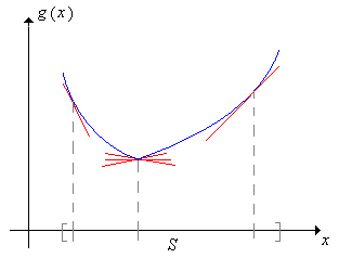
As with Jensen's inequality for ordinary expected value, the best proof uses the characterization of convex functions in terms of supporting lines: For each \( t \in S \) there exist numbers \( a \) and \( b \) (depending on \( t \)) such that
\( a + b t = g(t) \)
\( a + b x \le g(x) \) for \( x \in S \)
A convex function and several supporting lines
Random variables \( X \) and \( \E(X \mid \mathscr G) \) takes values in \( S \). We can construct a random supporting line at \( \E(X \mid \mathscr G) \). That is, there exist random variables \( A \) and \( B \), measurable with respect to \( \mathscr G \), such that
\( A + B \E(X \mid \mathscr G) = g[\E(X \mid \mathscr G)] \)
\( A + B X \le g(X) \)
We take conditional expected value through the inequality in (b) and then use properties of conditional expected value and property (a):
\[ \E[g(X) \mid \mathscr G] \ge \E(A + B X \mid \mathscr G) = A + B \E(X \mid \mathscr G) = g[\E(X \mid \mathscr G] \]
Note that the second step uses the fact that \( A \) and \( B \) are measurable with respect to \( \mathscr G \).
Conditional Probability
For our next discussion, suppose as usual that \( \mathscr G \) is a sub \( \sigma \)-algebra of \( \mathscr F \). The conditional probability of an event \(A\) given \( \mathscr G \) can be defined as a special case of conditional expected value. As usual, let \(\bs{1}_A\) denote the indicator random variable of \(A\).
For \( A \in \mathscr F \) we define
\[ \P(A \mid \mathscr G) = \E(\bs 1_A \mid \mathscr G) \]
Thus, we have the following characterizations of conditional probability, which are special cases of definition and the alternate version in :
If \( A \in \mathscr F \) then \( \P(A \mid \mathscr G) \) is characterized (up to equivalence) by the following properties
\( \P(A \mid \mathscr G) \) is measurable with respect to \( \mathscr G \).
If \( B \in \mathscr G \) then \( \E[\P(A \mid \mathscr G); B] = \P(A \cap B) \)
Details:
For part (b), note that
\[ \E[\bs{1}_B \P(A \mid \mathscr G)] = \E[\bs{1}_B \E(\bs{1}_A \mid
\mathscr G)] = \E(\bs{1}_A \bs{1}_B) = \E(\bs{1}_{A \cap B}) = \P(A \cap B) \]
If \( A \in \mathscr F \) then \( \P(A \mid \mathscr G) \) is characterized (up to equivalence) by the following properties
\( \P(A \mid \mathscr G) \) is measurable with respect to \( \mathscr G \).
If \( U \) is measurable with respect to \( \mathscr G \) and \( \E(|U|) \lt \infty \) then \( \E[U \P(A \mid \mathscr G)] = \E(U; A) \)
The properties above for conditional expected value, of course, have special cases for conditional probability. In particular, we can compute the probability of an event by conditioning on a \( \sigma \)-algebra:
If \( A \in \mathscr F \) then \(\P(A) = \E[\P(A \mid \mathscr G)]\).
Details:
This is a direct result of since \( \E(\bs{1}_A) = \P(A) \).
Again, is often a good way to compute \(\P(A)\) when we know the conditional probability of \(A\) given \(\mathscr G\). This is a very compact and elegant version of the law of total probability given first for events and later for discrete random variables. The following theorem gives the conditional version of the axioms of probability.
The following properties hold (as usual, modulo equivalence):
\( \P(A \mid \mathscr G) \ge 0 \) for every \( A \in \mathscr F \)
\( \P(\Omega \mid \mathscr G) = 1 \)
If \( \{A_i: i \in I\} \) is a countable disjoint subset of \( \mathscr F \) then \( \P(\bigcup_{i \in I} A_i \bigm| \mathscr G) = \sum_{i \in I} \P(A_i \mid \mathscr G) \)
Details:
This is a direct consequence of .
This is trivial since \( \bs{1}_\Omega = 1 \).
We show that the right side satisfies the conditions in that define the left side. Note that \( \sum_{i \in I} \P(A_i \mid \mathscr G) \) is \( \mathscr G \)-measurable since each term in the sum has this property. Let \( B \in \mathscr G \). then
\[ \E\left[\sum_{i \in I} \P(A_i \mid \mathscr G); B\right] = \sum_{i \in I} \E[\P(A_i \mid \mathscr G); B] = \sum_{i \in I} \P(A_i \cap B) = \P\left(B \cap \bigcup_{i \in I} A_i\right) \]
From , it follows that other standard probability rules hold for conditional probability given \( \mathscr G \) (as always, modulo equivalence). These results include
the complement rule
the increasing property
Boole's inequality
Bonferroni's inequality
the inclusion-exclusion laws
However, it is not correct to state that \( A \mapsto \P(A \mid \mathscr G) \) is a probability measure, because the conditional probabilities are only defined up to equivalence, and so the mapping does not make sense. We would have to specify a particular version of \( \E(A \mid \mathscr G) \) for each \( A \in \mathscr F \) for the mapping to make sense. Even if we do this, the mapping may not define a probability measure. In part (c), the left and right sides are random variables and the equation is an event that has probability 1. However this event depends on the collection \( \{A_i: i \in I\} \). In general, there will be uncountably many such collections in \( \mathscr F \), and the intersection of all of the corresponding events may well have probability less than 1 (if it's measurable at all). It turns out that if the underlying probability space \( (\Omega, \mathscr F, \P) \) is sufficiently nice (and most probability spaces that arise in applications are nice), then there does in fact exist a regular conditional probability. That is, for each \( A \in \mathscr F \), there exists a random variable \( \P(A \mid \mathscr G) \) satisfying the conditions in and such that with probability 1, \( A \mapsto \P(A \mid \mathscr G) \) is a probability measure.
The following theorem gives a version of Bayes' theorem, named for the inimitable Thomas Bayes.
Suppose that \( A \in \mathscr G \) and \( B \in \mathscr F \). then
\[ \P(A \mid B) = \frac{\E[\P(B \mid \mathscr G); A]}{\E[\P(B \mid \mathscr G)]} \]
Details:
The proof is absolutely trivial. By definition of conditional probability given \( \mathscr G \), the numerator is \( \P(A \cap B) \) and the denominator is \( P(B) \). Nonetheless, Bayes' theorem is useful in settings where the expected values in the numerator and denominator can be computed directly
Basic Examples
The purpose of this discussion is to tie the general notions of conditional expected value that we are studying here to the more elementary concepts that you have seen before. Suppose that \( A \) is an event (that is, a member of \( \mathscr F \)) with \( \P(A) \gt 0 \). If \( B \) is another event, then the conditional probability of \( B \) given \( A \) is
\[ \P(B \mid A) = \frac{\P(A \cap B)}{\P(A)} \]
If \( X \) is a random variable then the conditional distribution of \( X \) given \( A \) is the probability measure on \( \R \) given by
\[ R \mapsto \P(X \in R \mid A) = \frac{\P(\{X \in R\} \cap A)}{\P(A)} \text{ for measurable } R \subseteq \R \]
If \( \E(|X|) \lt \infty \) then the conditional expected value of \( X \) given \( A \), denoted \( \E(X \mid A) \), is simply the mean of this conditional distribution.
Suppose now that \( \mathscr{A} = \{A_i: i \in I\} \) is a countable partition of the sample space \( \Omega \) into events with positive probability. To review the jargon, \( \mathscr A \subseteq \mathscr F \); the index set \( I \) is countable; \( A_i \cap A_j = \emptyset \) for distinct \( i, \, j \in I \); \( \bigcup_{i \in I} A_i = \Omega \); and \( \P(A_i) \gt 0 \) for \( i \in I \). Let \( \mathscr G = \sigma(\mathscr{A}) \), the \( \sigma \)-algebra generated by \( \mathscr{A} \). The elements of \( \mathscr G \) are of the form \( \bigcup_{j \in J} A_j \) for \( J \subseteq I \). Moreover, the random variables that are measurable with respect to \( \mathscr G \) are precisely the variables that are constant on \( A_i \) for each \( i \in I \). The \( \sigma \)-algebra \( \mathscr G \) is said to be countably generated.
If \( B \in \mathscr F \) then \( \P(B \mid \mathscr G) \) is the random variable whose value on \( A_i \) is \( \P(B \mid A_i) \) for each \(i \in I \).
Details:
Let \( U \) denote the random variable that takes the value \( \P(B \mid A_i) \) on \( A_i \) for each \( i \in I \). First, \( U \) is measurable with respect to \( \scr G \) since \( U \) is constant on \( A_i \) for each \( i \in I \). So we just need to show that \( E(U ; A) = \P(A \cap B) \) for each \( A \in \mathscr G \). Thus, let \( A = \bigcup_{j \in J} A_j \) where \( J \subseteq I \). Then
\[ \E(U; A) = \sum_{j \in J} \E(U ; A_j) = \sum_{j \in J} \P(B \mid A_j) \P(A_j) = \P(A \cap B)\]
In this setting, the version of Bayes' theorem reduces to the usual elementary formulation: For \( i \in I \), \( \E[\P(B \mid \mathscr G); A_i] = \P(A_i) \P(B \mid A_i) \) and \( \E[\P(B \mid \mathscr G)] = \sum_{j \in I} \P(A_j) \P(B \mid A_j) \). Hence
\[ \P(A_i \mid B) = \frac{\P(A_i) \P(B \mid A_i)}{\sum_{j \in I} \P(A_j) \P(B \mid A_j)} \]
If \( X \) is a random variable with \( \E(|X|) \lt \infty \), then \( \E(X \mid \mathscr G) \) is the random variable whose value on \( A_i \) is \( \E(X \mid A_i) \) for each \( i \in I \).
Details:
Let \( U \) denote the random variable that takes the value \( \E(X \mid A_i) \) on \( A_i \) for each \( i \in I \). First, \( U \) is measurable with respect to \( \scr G \) since \( U \) is constant on \( A_i \) for each \( i \in I \). So we just need to show that \( E(U; A) = \E(X; A) \) for each \( A \in \mathscr G \). Thus, let \( A = \bigcup_{j \in J} A_j \) where \( J \subseteq I \). Then
\[ \E(U; A) = \sum_{j \in J} \E(U; A_j) = \sum_{j \in J} \E(X \mid A_j) \P(A_j) = E(X; A) \]
Example and example would apply to \( \mathscr G = \sigma(Y) \) if \( Y \) is a discrete random variable with values in a countable set \( T \). In this case, the partition is simply \( \mathscr{A} = \{ \{Y = y\}: y \in T\} \). On the other hand, suppose that \( Y \) is a random variable taking values in a general set \( T \) with \( \sigma \)-algebra \( \mathscr{T} \). The real-valued random variables that are measurable with respect to \( \mathscr G = \sigma(Y) \) are (up to equivalence) the measurable, real-valued functions of \( Y \).
Specializing further, Suppose that \( X \) takes values in \( S \subseteq \R \), \( Y \) takes values in \( T \subseteq \R^n \) (where \( S \) and \( T \) are Lebesgue measurable) and that \( (X, Y) \) has a joint continuous distribution with probability density function \( f \). Then \( Y \) has probability density function \( h \) given by
\[ h(y) = \int_S f(x, y) \, dx, \quad y \in T \]
Assume that \( h(y) \gt 0 \) for \( y \in T \). Then for \( y \in T \), a conditional probability density function of \( X \) given \( Y = y \) is defined by
\[ g(x \mid y) =\frac{f(x, y)}{h(y)}, \quad x \in S \]
This is precisely the setting of our elementary discussion of conditional expected value. If \( \E(|X|) \lt \infty \) then we usually write \( \E(X \mid Y) \) instead of the clunkier \( \E[X \mid \sigma(Y)] \).
In this setting above suppose that \( \E(|X|) \lt \infty \). Then
\[ \E(X \mid Y) = \int_S x g(x \mid Y) \, dx \]
Details:
Once again, we show that the integral on the right satisfies the properties in the definition in for \( \E(X \mid Y) = \E[X \mid \sigma(Y)] \). First, \( y \mapsto \int_S x g(x \mid y) \, dx \) is measurable as a function from \( T \) into \( \R \) and hence the random variable \( \int_x g(x \mid Y) \, dx \) is a measurable function of \( Y \) and so is measurable with respect to \( \sigma (Y) \). Next suppose that \( B \in \sigma(Y) \). Then \( B = \{Y \in A\} \) for some \( A \in \mathscr F \). Then
\begin{align*}
\E\left[\int_S x g(x \mid Y) \, dx; B\right] & = \E\left[\int_S x g(x \mid Y) \, dx; Y \in A\right] \\
& = \E\left[\int_S x \frac{f(x, y)}{h(y)} \, dx; Y \in A\right] = \int_A \int_S x \frac{f(x, y)}{h(y)} h(y) \, dx \, dy \\
& = \int_{S \times A} x f(x, y) \, d(x, y) = \E(X; Y \in A) = \E(X; B)
\end{align*}
Best Predictor
In our elementary treatment of conditional expected, we showed that the conditional expected value of a real-valued random variable \( X \) given a general random variable \( Y \) is the best predictor of \( X \), in the least squares sense, among all real-valued functions of \( Y \). A more careful statement is that \( \E(X \mid Y) \) is the best predictor of \( X \) among all real-valued random variables that are measurable with respect to \( \sigma(Y) \). Thus, it should come as not surprise that if \( \mathscr G \) is a sub \( \sigma \)-algebra of \( \mathscr F \), then \( \E(X \mid \mathscr G) \) is the best predictor of \( X \), in the least squares sense, among all real-valued random variables that are measurable with respect to \( \mathscr G) \). We will show that this is indeed the case in this subsection. The proofs are very similar to the ones given in the elementary section. For the rest of this discussion, we assume that \( \mathscr G \) is a sub \( \sigma \)-algebra of \( \mathscr F \) and that all random variables mentioned are real valued.
Suppose that \( X \) and \( U \) are random variables with \( \E(|X|) \lt \infty \) and \( \E(|X U|) \lt \infty \) and that \( U \) is measurable with respect to \( \mathscr G \). Then \( X - \E(X \mid \mathscr G) \) and \( U \) are uncorrelated.
Details:
Note that \( X - \E(X \mid \mathscr G) \) has mean 0 by the mean property in . Using the properties that characterize in \( \E(X \mid \mathscr G) \) we have
\[ \cov[X - \E(X \mid \mathscr G), U] = \E(U [X - \E(X \mid \mathscr G)]) = \E(U X) - \E[U \E(X \mid \mathscr G] = \E(U X) - \E(U X) = 0 \]
The next result is the main one: \( \E(X \mid \mathscr G) \) is closer to \( X \) in the mean square sense than any other random variable that is measurable with respect to \( \mathscr G \). Thus, if \( \mathscr G \) represents the information that we have, then \( \E(X \mid \mathscr G) \) is the best we can do in estimating \( X \).
Suppose that \( X \) and \( U \) are random variables with \( \E(X^2) \lt \infty \) and \( \E(U^2) \lt \infty\) and that \( U \) is measurable with respect to \( \mathscr G \). Then
Equality holds if and only if \(\P[U = \E(X \mid \mathscr G)] = 1 \), so \( U \) and \( \E(X \mid \mathscr G) \) are equivalent.
Details:
Note that
\begin{align}
\E[(X - U)^2] & = \E([X - \E(X \mid \mathscr G) + \E(X \mid \mathscr G) - U]^2) \\
& = \E([X - \E(X \mid \mathscr G)]^2) + 2 \E([X - \E(X \mid \mathscr G)][\E(X \mid \mathscr G) - U]) + \E([\E(X \mid \mathscr G) - U]^2 )
\end{align}
By , \( X - \E(X \mid \mathscr G) \) has mean 0, so the middle term in the displayed equation is \( 2 \cov[X - \E(X \mid \mathscr G), \E(X \mid \mathscr G) - U] \). But \( \E(X \mid \mathscr G) - U \) is \( \mathscr G \)-measurable and hence this covariance is 0 by . Therefore
\[ \E[(X - U)^2] = \E([X - \E(X \mid \mathscr G)]^2) + \E([\E(X \mid \mathscr G) - U]^2 ) \ge \E([X - \E(X \mid \mathscr G)]^2) \]
Equality holds if and only if \( \E([\E(X \mid \mathscr G) - U]^2 ) = 0 \) if and only if \(\P[U = \E(X \mid \mathscr G)] = 1 \)
Conditional Variance
Once again, we assume that \( \mathscr G \) is a sub \( \sigma \)-algebra of \( \mathscr F \) and that all random variables mentioned are real valued, unless otherwise noted. It's natural to define the conditional variance of a random variable given \( \mathscr G \) in the same way as ordinary variance, but witl all expected values conditioned on \( \mathscr G \).
Suppose that \( X \) is a random variable with \( \E(X^2) \lt \infty \). The conditional variance of \( X \) given \(\mathscr G\) is
\[ \var(X \mid \mathscr G) = \E\left([X - \E(X \mid \mathscr G)]^2 \biggm| \mathscr G\right) \]
Like all conditional expected values relative to \( \mathscr G \), \( \var(X \mid \mathscr G) \) is a random variable that is measurable with respect to \( \mathscr G \) and is unique up to equivalence. The first property is analogous to the computational formula for ordinary variance.
Suppose again that \( X \) is a random variable with \( \E(X^2) \lt \infty \). Then
\[\var(X \mid \mathscr G) = \E(X^2 \mid \mathscr G) - [\E(X \mid \mathscr G)]^2\]
Details:
Expanding the square in the definition and using basic properties of conditional expectation, we have
Next is a formula for the ordinary variance in terms of conditional variance and expected value.
Suppose again that \( X \) is a random variable with \( \E(X^2) \lt \infty \). Then
\[\var(X) = \E[\var(X \mid \mathscr G)] + \var[\E(X \mid \mathscr G)]\]
Details:
From and properties of conditional expected value we have \( \E[\var(X \mid \mathscr G)] = \E(X^2) - \E([\E(X \mid \mathscr G)]^2) \). But \( \E(X^2) = \var(X) + [\E(X)]^2 \) and similarly, \(\E([\E(X \mid \mathscr G)]^2) = \var[\E(X \mid \mathscr G)] + (\E[\E(X \mid \mathscr G)])^2 \). But also, \( \E[\E(X \mid \mathscr G)] = \E(X) \) so subsituting we get \( \E[\var(X \mid \mathscr G)] = \var(X) - \var[\E(X \mid \mathscr G)] \).
So the variance of \( X \) is the expected conditional variance plus the variance of the conditional expected value. This result is often a good way to compute \(\var(X)\) when we know the conditional distribution of \(X\) given \(\mathscr G\). In turn, this property leads to a formula for the mean square error when \( \E(X \mid \mathscr G) \) is thought of as a predictor of \( X \).
Suppose again that \( X \) is a random variable with \( \E(X^2) \lt \infty \).
\[ \E([X - \E(X \mid \mathscr G)]^2) = \var(X) - \var[\E(X \mid \mathscr G)] \]
Details:
From the definition and from and ,
\[ \E([X - \E(X \mid \mathscr G)]^2) = \E[\var(X \mid \mathscr G)] = \var(X) - \var[\E(X \mid \mathscr G)] \]
Let us return to the study of predictors of the real-valued random variable \(X\), and compare them in terms of mean square error.
Suppose again that \( X \) is a random variable with \( \E(X^2) \lt \infty \).
The best constant predictor of \(X\) is \(\E(X)\) with mean square error \(\var(X)\).
If \(Y\) is another random variable with \( \E(Y^2) \lt \infty \), then the best predictor of \(X\) among linear functions of \(Y\) is
\[ L(X \mid Y) = \E(X) + \frac{\cov(X,Y)}{\var(Y)}[Y - \E(Y)] \]
with mean square error \( \var(X)[1 - \cor^2(X,Y)]\).
If \(Y\) is a (general) random variable, then the best predictor of \(X\) among all real-valued functions of \(Y\) with finite variance is \(\E(X \mid Y)\) with mean square error \( \var(X) - \var[\E(X \mid Y)]\).
If \(\mathscr G\) is a sub \( \sigma \)-algebra of \( \mathscr F \), then the best predictor of \(X\) among random variables with finite variance that are measurable with respect to \(\mathscr G\) is \(\E(X \mid \mathscr G)\) with mean square error \(\var(X) - \var[\E(X \mid \mathscr G)]\).
Of course, (a) is a special case of (d) with \( \mathscr G = \{\emptyset, \Omega\} \) and (c) is a special case of (d) with \( \mathscr G = \sigma(Y) \). Only (b), the linear case, cannot be interpreted in terms of conditioning with respect to a \( \sigma \)-algebra.
Conditional Covariance
Suppose again that \( \mathscr G \) is a sub \( \sigma \)-algebra of \( \mathscr F \). The conditional covariance of two random variables is defined like the ordinary covariance, but with all expected values conditioned on \( \mathscr G \).
Suppose that \( X \) and \( Y \) are random variables with \( \E(X^2) \lt \infty \) and \( \E(Y^2) \lt \infty \). The conditional covariance of \(X\) and \( Y \) given \(\mathscr G\) is defined as
\[ \cov(X, Y \mid \mathscr G) = \E\left([X - \E(X \mid \mathscr G)] [Y - \E(Y \mid \mathscr G)] \biggm| \mathscr G \right) \]
So \( \cov(X, Y \mid \mathscr G) \) is a random variable that is measurable with respect to \( \mathscr G \) and is unique up to equivalence. As should be the case, conditional covariance generalizes conditional variance.
Suppose that \( X \) is a random variable with \( \E(X^2) \lt \infty \). Then \( \cov(X, X \mid \mathscr G) = \var(X \mid \mathscr G) \).
Details:
This follows immediately from definition . and definition
Our next result is a computational formula that is analogous to the one for standard covariance—the covariance is the mean of the product minus the product of the means, but now with all expected values conditioned on \( \mathscr G \):
Suppose again that \( X \) and \( Y \) are random variables with \( \E(X^2) \lt \infty \) and \( \E(Y^2) \lt \infty \). Then
\[\cov(X, Y \mid \mathscr G) = \E(X Y \mid \mathscr G) - \E(X \mid \mathscr G) E(Y \mid \mathscr G)\]
Details:
Expanding the product in the definition and using basic properties of conditional expectation, we have
Our next result shows how to compute the ordinary covariance of \( X \) and \( Y \) by conditioning on \( X \).
Suppose again that \( X \) and \( Y \) are random variables with \( \E(X^2) \lt \infty) \) and \( \E(Y^2 \lt \infty) \). Then
\[\cov(X, Y) = \E\left[\cov(X, Y \mid \mathscr G)\right] + \cov\left[\E(X \mid \mathscr G), \E(Y \mid \mathscr G) \right]\]
Details:
From (29) and properties of conditional expected value we have
\[ \E\left[\cov(X, Y \mid \mathscr G)\right] = \E(X Y) - \E\left[\E(X\mid \mathscr G) \E(Y \mid \mathscr G) \right] \]
But \( \E(X Y) = \cov(X, Y) + \E(X) \E(Y)\) and similarly,
\[\E\left[\E(X \mid \mathscr G) \E(Y \mid \mathscr G)\right] = \cov[\E(X \mid \mathscr G), \E(Y \mid \mathscr G) + \E[\E(X\mid \mathscr G)] \E[\E(Y \mid \mathscr G)]\]
But also, \( \E\left[\E(X \mid \mathscr G)\right] = \E(X) \) and \( \E[\E(Y \mid \mathscr G)] = \E(Y) \) so subsituting we get
\[ \E\left[\cov(X, Y \mid \mathscr G)\right] = \cov(X, Y) - \cov\left[\E(X \mid \mathscr G), \E(Y \mid \mathscr G)\right] \]
So the covariance of \( X \) and \( Y \) is the expected conditional covariance plus the covariance of the conditional expected values. This result is often a good way to compute \(\cov(X, Y)\) when we know the conditional distribution of \((X, Y)\) given \(\mathscr G\).