Suppose that we have a sequence of trials, each of which results in either success or failure. Our basic assumption is that if there have been \( x \in \N \) consecutive successes, then the probability of success on the next trial is \( p(x) \), independently of the past, where \( p: \N \to (0, 1) \). Whenever there is a failure, we start over, independently, with a new sequence of trials. Appropriately enough, \( p \) is called the success function. Let \( X_n \) denote the length of the run of successes after \( n \) trials.
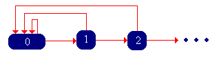
\( \bs{X} =(X_0, X_1, X_2, \ldots) \) is a discrete-time Markov chain with state space \( \N \) and transition probability matrix \( P \) given by \[ P(x, x + 1) = p(x), \; P(x, 0) = 1 - p(x); \quad x \in \N \] The Markov chain \( \bs{X} \) is called the success-runs chain.
Now let \( T \) denote the trial number of the first failure, starting with a fresh sequence of trials. Note that in the context of the success-runs chain \( \bs{X} \), \( T = \tau_0 \), the first return time to state 0, starting in 0. Note that \( T \) takes values in \( \N_+ \cup \{\infty\} \), since presumably, it is possible that no failure occurs. Let \( r(n) = \P(T \gt n) \) for \( n \in \N \), the probability of at least \( n \) consecutive successes, starting with a fresh set of trials. Let \( f(n) = \P(T = n + 1) \) for \( n \in \N \), the probability of exactly \( n \) consecutive successes, starting with a fresh set of trails.
The functions \( p \), \( r \), and \( f \) are related as follows:
Thus, the functions \( p \), \( r \), and \( f \) give equivalent information. If we know one of the functions, we can construct the other two, and hence any of the functions can be used to define the success-runs chain. The function \( r \) is the reliability function associated with \( T \).
The function \( r \) is characterized by the following properties:
The function \( f \) is characterized by the following properties:
Essentially, \( f \) is the probability density function of \( T - 1 \), except that it may be defective in the sense that the sum of its values may be less than 1. The leftover probability, of course, is the probability that \( T = \infty \). This is the critical consideration in the classification of the success-runs chain, which we will consider shortly.
Verify that each of the following functions has the appropriate properties, and then find the other two functions:
In part (a) of , note that the trials are Bernoulli Trials. We have an app for this case.
The success-runs app is a simulation of the success-runs chain based on Bernoulli trials. Run the simulation 1000 times for various values of \( p \) and various initial states, and note the general behavior of the chain.
The success-runs chain is irreducible and aperiodic.
The chain is irreducible, since 0 leads to every other state, and every state leads back to 0. The chain is aperiodic since \( P(0, 0) \gt 0 \).
Recall that \( T \) has the same distribution as \( \tau_0 \), the first return time to 0 starting at state 0. Thus, the classification of the chain as recurrent or transient depends on \( \alpha = \P(T = \infty) \). Specifically, the success-runs chain is transient if \( \alpha \gt 0 \) and recurrent if \( \alpha = 0 \). Thus, we see that the chain is recurrent if and only if a failure is sure to occur. We can compute the parameter \( \alpha \) in terms of each of the three functions that define the chain.
In terms of \( p \), \( r \), and \( f \), \[ \alpha = \prod_{x=0}^\infty p(x) = \lim_{n \to \infty} r(n) = 1 - \sum_{x=0}^\infty f(x) \]
Compute \( \alpha \) and determine whether the success-runs chain \( \bs{X} \) is transient or recurrent for each of the examples in .
Run the simulation of the success-runs chain 1000 times for various values of \( p \), starting in state 0. Note the return times to state 0.
Let \( \mu = \E(T) \), the expected trial number of the first failure, starting with a fresh sequence of trials.
\( \mu \) is related to \( \alpha \), \( f \), and \( r \) as follows:
The success-runs chain \( \bs{X} \) is positive recurrent if and only if \( \mu \lt \infty \).
Since \( T \) is the return time to 0, starting at 0, and since the chain is irreducible, it follows from the general theory that the chain is positive recurrent if and only if \( \mu = \E(T) \lt \infty \).
If \( \bs{X} \) is recurrent, then \( r \) is invariant for \( \bs{X} \). In the positive recurrent case, when \( \mu \lt \infty \), the invariant distribution has probability density function \( g \) given by \[ g(x) = \frac{r(x)}{\mu}, \quad x \in \N \]
If \( y \in \N_+ \) then from , \[(r P)(y) = \sum_{x=0}^\infty r(x) P(x, y) = r(y - 1) p(y - 1) = r(y)\] For \( y = 0 \), using again, \[(r P)(0) = \sum_{x=0}^\infty r(x) P(x, 0) = \sum_{x=0}^\infty r(x)[1 - p(x)] = \sum_{x=0}^\infty [r(x) - r(x)p(x)] = \sum_{x=0}^\infty [r(x) - r(x + 1)]\] If the chain is recurrent, \( r(n) \to 0 \) as \( n \to \infty \) so the last sum collapses to \( r(0) = 1 \). Recall that \( \mu = \sum_{n = 0}^\infty r(n) \). Hence if \( \mu \lt \infty \), so that the chain is positive recurrent, the function \( g \) (which is just \( r \) normalized) is the invariant PDF.
When \( \bs{X} \) is recurrent, we know from the general theory that every other nonnegative left invariant function is a nonnegative multiple of \( r \)
Determine whether the success-runs chain \( \bs{X} \) is transient, null recurrent, or positive recurrent for each of the examples in . If the chain is positive recurrent, find the invariant probability density function.
From part (a) of , the success-runs chain corresponding to Bernoulli trials with success probability \( p \in (0, 1) \) has the geometric distribution on \( \N \), with parameter \( 1 - p \), as the invariant distribution.
Run the simulation of the success-runs chain 1000 times for various values of \( p \) and various initial states. Compare the empirical distribution to the invariant distribution.
Consider a device whose (discrete) time to failure \( U \) takes values in \( \N \), with probability density function \( f \). We assume that \( f(n) \gt 0 \) for \( n \in \N \). When the device fails, it is immediately (and independently) replaced by an identical device. For \( n \in \N \), let \( Y_n \) denote the time to failure of the device that is in service at time \( n \).
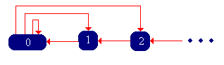
\( \bs{Y} = (Y_0, Y_1, Y_2, \ldots) \) is a discrete-time Markov chain with state space \( \N \) and transition probability matrix \( Q \) given by \[ Q(0, x) = f(x), \; Q(x + 1, x) = 1; \quad x \in \N \]
The Markov chain \( \bs{Y} \) is called the remaining life chain with lifetime probability density function \( f \), and has the state graph below.
We have an app for the remaining life chain whose lifetime distribution is the geometric distribution on \( \N \), with parameter \( 1 - p \in (0, 1) \).
Run the simulation of the remaining-life chain 1000 times for various values of \( p \) and various initial states. Note the general behavior of the chain.
If \( U \) denotes the lifetime of a device, as before, note that \( T = 1 + U \) is the return time to 0 for the chain \( \bs{Y} \), starting at 0.
\( \bs{Y} \) is irreducible, aperiodic, and recurrent.
From the assumptions on \( f \), state 0 leads to every other state (including 0), and every positive state leads (deterministically) to 0. Thus the chain is irreducible and aperiodic. By assumption, \( \P(U \in \N) = 1 \) so \( \P(T \lt \infty) = 1 \) and hence the chain is recurrent.
Now let \( r(n) = \P(U \ge n) = \P(T \gt n) \) for \( n \in \N \) and let \( \mu = \E(T) = 1 + \E(U) \). Note that \( r(n) = \sum_{x=n}^\infty f(x) \) and \( \mu = 1 + \sum_{x=0}^\infty f(x) = \sum_{n=0}^\infty r(n) \).
The success-runs chain \( \bs{X} \) is positive recurrent if and only if \( \mu \lt \infty \), in which case the invariant distribution has probability density function \( g \) given by \[ g(x) = \frac{r(x)}{\mu}, \quad x \in \N \]
Since the chain is irreducible, it is positive recurrent if and only if \( \mu = E(T) \lt \infty \). The function \( r \) is invariant for \( Q \): for \( y \in \N \) \begin{align*} (r Q)(y) &= \sum_{x \in \N} r(x) Q(x, y) = r(0) Q(0, y) + r(y + 1) Q(y + 1, y) \\ &= f(y) + r(y + 1) = r(y) \end{align*} In the positive recurrent case, \( \mu \) is the normalizing constant for \( r \), so \( g \) is the invariant PDF.
Suppose that \( \bs{Y} \) is the remaining life chain whose lifetime distribution is the geometric distribution on \( \N \) with parameter \( 1 - p \in (0, 1) \). Then this distribution is also the invariant distribution.
By assumption, \( f(x) = (1 - p) p^x \) for \( x \in \N \), and the mean of this distribution is \( p / (1 - p) \). Hence \( \mu = 1 + p / (1 - p) = 1 / (1 - p) \), and \( r(x) = \sum_{y = x}^\infty f(y) = p^x \) for \( x \in \N \). Hence \( g = f \).
Run the simulation of the success-runs chain 1000 times for various values of \( p \) and various initial states. Compare the empirical distribution to the invariant distribution.
You probably have already noticed similarities, in notation and results, between the success-runs chain and the remaining-life chain. There are deeper connections.
Suppose that \( f \) is a probability density function on \( \N \) with \( f(n) \gt 0 \) for \( n \in \N \). Let \( \bs{X} \) be the success-runs chain associated with \( f \) and \( \bs{Y} \) the remaining life chain associated with \( f \). Then \( \bs{X} \) and \( \bs{Y} \) are time reversals of each other.
Under the assumptions on \( f \), both chains are recurrent and irreducible. Hence it suffices to show that \[ r(x) P(x, y) = r(y) Q(y, x), \quad x, \, y \in \N \] It will then follow that the chains are time reversals of each other, and that \( r \) is a common invariant function (unique up to multiplication by positive constants). In the case that \( \mu = \sum_{n=0}^\infty r(n) \lt \infty \), the function \( g = r / \mu \) is the common invariant PDF. There are only two cases to consider. With \( y = 0 \), we have \( r(x) P(x, 0) = r(x)[1 - p(x)] \) and \( r(0) Q(y, 0) = f(x) \). But \( r(x) [1 - p(x)] = f(x) \) by . When \( x \in \N \) and \( y = x + 1 \), we have \( r(x) P(x, x + 1) = r(x) p(x) \) and \( r(x + 1) Q(x + 1, x) = r(x + 1) \). But \( r(x) p(x) = r(x + 1) \) by .
In the context of reliability, it is also easy to see that the chains are time reversals of each other. Consider again a device whose random lifetime takes values in \( \N \), with the device immediately replaced by an identical device upon failure. For \( n \in \N \), we can think of \( X_n \) as the age of the device in service at time \( n \) and \( Y_n \) as the time remaining until failure for that device.
Open the simulation of the success-runs chain and the simulaiton of the remaining-life chain. Run the two simulations 1000 times for the same values of \( p \), starting in state 0 and note the time reversal.