Recall that with the strategy of bold play in red and black, the gambler on each game bets either her entire fortune or the amount needed to reach the target fortune, whichever is smaller. As usual, we are interested in the probability that the player reaches the target and the expected number of trials. The first interesting fact is that only the ratio of the initial fortune to the target fortune matters, quite in contrast to timid play.
Suppose that the gambler plays boldly with initial fortune \(x\) and target fortune \(a\). As usual, let \(\bs{X} = (X_1, X_2, \ldots)\) denote the fortune process for the gambler. For any \(c \gt 0\), the random process \(c \bs{X} = (c X_0, c X_1, \ldots)\) is the fortune process for bold play with initial fortune \(c x\) and target fortune \(c a\).
Because of , it is convenient to use the target fortune as the monetary unit and to allow irrational, as well as rational, initial fortunes. Thus, the fortune space is \([0, 1]\). Sometimes in our analysis we will ignore the states 0 or 1; clearly there is no harm in this because in these states, the game is over.
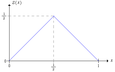
Recall that the betting function \(S\) is the function that gives the amount bet as a function of the current fortune. For bold play, the betting function is \[ S(x) = \min\{x, 1 - x\} = \begin{cases} x, & 0 \le x \le \frac{1}{2} \\ 1 - x, & \frac{1}{2} \le x \le 1 \end{cases} \]
We will denote the probability that the bold gambler reaches the target \(a = 1\) starting from the initial fortune \(x \in [0, 1]\) by \(F(x)\). By the scaling property in , the probability that the bold gambler reaches some other target value \(a \gt 0\), starting from \(x \in [0, a]\) is \(F(x / a)\).
The function \(F\) satisfies the following functional equation and boundary conditions:
From , and a little thought, it should be clear that an important role is played by the following function:
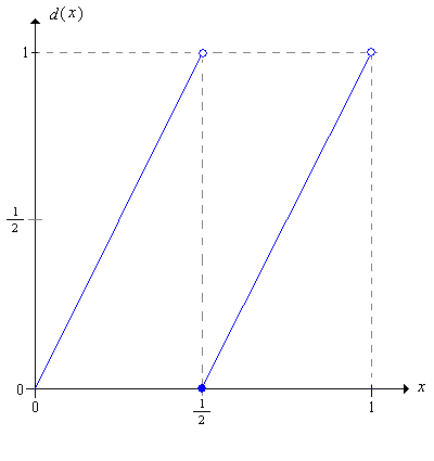
Let \(d\) be the function defined on \([0, 1)\) by \[ d(x) = 2 x - \lfloor 2 x \rfloor = \begin{cases} 2 x, & 0 \le x \lt \frac{1}{2} \\ 2 x - 1, & \frac{1}{2} \le x \lt 1 \end{cases} \] The function \(d\) is called the doubling function, mod 1, since \(d(x)\) gives the fractional part of \(2 x\).
Note that until the last bet that ends the game (with the player ruined or victorious), the successive fortunes of the player follow iterates of the map \(d\). Thus, bold play is intimately connected with the dynamical system associated with \(d\).
One of the keys to our analysis is to represent the initial fortune in binary form.
The binary expansion of \(x \in [0, 1)\) is \[ x = \sum_{i=1}^\infty \frac{x_i}{2^i} \] where \(x_i \in \{0, 1\}\) for each \(i \in \N_+\). This representation is unique except when \(x\) is a binary rational (sometimes also called a dyadic rational), that is, a number of the form \(k / 2^n\) where \(n \in \N_+\) and \(k \in \{1, 3, \ldots, 2^n - 1\}\); the positive integer \(n\) is called the rank of \(x\).
For a binary rational \(x\) of rank \(n\), we will use the standard terminating representation where \(x_n = 1\) and \(x_i = 0\) for \(i \gt n\). Rank can be extended to all numbers in [0, 1) by defining the rank of 0 to be 0 (0 is also considered a binary rational) and by defining the rank of a binary irrational to be \(\infty\). We will denote the rank of \(x\) by \(r(x)\).
Applied to the binary sequences, the doubling function \(d\) is the shift operator:
For \(x \in [0, 1)\), \( [d(x)]_i = x_{i+1} \).
Bold play in red and black can be elegantly described by comparing the bits of the initial fortune with the game bits.
Suppose that gambler starts with initial fortune \(x \in (0, 1)\). The player wins after \(k \in \N_+\) trials if and only if \(I_j = 1 - x_j\) for \(j \in \{1, 2, \ldots, k - 1\}\) and \(I_k = x_k = 1\).
The random variable whose bits are the complements of the fortune bits will play an important role in our analysis. Thus, let \[ W = \sum_{j=1}^\infty \frac{1 - I_j}{2^j} \]
Note that \(W\) is a well defined random variable taking values in \([0, 1]\).
Suppose that the gambler starts with initial fortune \(x \in (0, 1)\). Then the gambler reaches the target 1 if and only if \(W \lt x\).
\(W\) has a continuous distribution. That is, \(\P(W = x) = 0\) for any \(x \in [0, 1]\).
From and , it follows that \(F\) is simply the distribution function of \(W\). In particular, \(F\) is an increasing function, and since \(W\) has a continuous distribution, \(F\) is a continuous function.
The success function \(F\) is the unique continuous solution of the functional equation in .
Induction on the rank shows that any two solutions must agree at the binary rationals. But then any two continuous solutions must agree for all \(x \in [0, 1]\).
If we introduce a bit more notation, we can give nice expression for \(F(x)\), and later for the expected number of games \(G(x)\). Let \(p_0 = p\) and \(p_1 = q = 1 - p\).
The win probability function \(F\) can be expressed as follows: \[ F(x) = \sum_{n=1}^\infty p_{x_1} \cdots p_{x_{n-1}} p x_n \]
Note that \( p \cdot x_n \) in the last expression is correct; it's not a misprint of \( p_{x_n} \). Thus, only terms with \( x_n = 1 \) are included in the sum.
\(F\) is strictly increasing on \([0, 1]\). This means that the distribution of \(W\) has support \([0, 1]\); that is, there are no subintervals of \([0, 1]\) that have positive length, but 0 probability.
In particular,
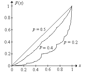
If \(p = \frac{1}{2}\) then \(F(x) = x\) for \(x \in [0, 1]\)
So for \(p = \frac{1}{2}\) (fair trials), the probability that the bold gambler reaches the target fortune \(a\) starting from the initial fortune \(x\) is \(x / a\), just as it is for the timid gambler. Note also that the random variable \(W\) has the uniform distribution on \([0, 1]\). When \(p \ne \frac{1}{2}\), the distribution of \(W\) is quite strange. To state the result succinctly, we will indicate the dependence of the of the probability measure \(\P\) on the parameter \(p \in (0, 1)\). First we define \[ C_p = \left\{ x \in [0, 1]: \frac{1}{n} \sum_{i=1}^n (1 - x_i) \to p \text{ as } n \to \infty \right\} \] So \(C_p\) is the set of \(x \in [0, 1]\) for which the relative frequency of 0's in the binary expansion is \(p\).
For distinct \(p, \, t \in (0, 1)\)
Part (a) follows from the strong law of large numbers. Part (b) follows from part (a) since \(C_p \cap C_t = \emptyset\).
When \(p \ne \frac{1}{2}\), \(W\) does not have a probability density function (with respect to Lebesgue measure on [0, 1]), even though \(W\) has a continuous distribution.
The proof is by contradiction. Suppose that \(W\) has probability density function \(f\). Then \( 1 = \P_p(W \in C_p) = \int_{C_p} f(x) \, dx \). But if \( p \ne \frac{1}{2} \), \( \int_{C_p} 1 \, dx = \P_{1/2}(W \in C_p) = 0 \). That is, \(C_p\) has Lebesgue measure 0. But then \(\int_{C_p} f(x) \, dx = 0\), a contradiction.
When \(p \ne \frac{1}{2}\), \(F\) has derivative 0 at almost every point in \([0, 1]\), even though it is strictly increasing.
Open the bold play experiment. Vary the initial fortune, target fortune, and trial probability with the input controls, and note how the probability of winning the game changes. In particular, note that this probability depends only on \(x / a\). Now for various values of the parameters, run the experiment 1000 times and compare the relative frequency of wins to the probability of winning.
As usual, let \(N\) denote the number of trials so that \(N = \min\{n \in \N_+: X_n \in \{0, 1\}\}\) where \(\bs{X} = (X_0, X_1, \ldots)\) is the sequence of fortunes. The distribution of \(N\) is complicated, but once again the binary representation of the initial fortune gives some insight.
Suppose that the initial fortune of the gambler is \(x \in (0, 1)\). Then \(N = \min\{k \in \N_+: I_k = x_k \text{ or } k = r(x)\}\).
Open the bold play experiment. Vary the target fortune and initial fortune and note the set of values of \(N\). For various values of the parameters, run the experiment 1000 times and note the shape and location of the empirical density function of \(N\).
As with timid play, our primary interest is in the expected number of trials as a function of the initial fortune. Thus, let \(G(x) = \E(N \mid X_0 = x)\) for \(x \in [0, 1]\). For any other target fortune \(a \gt 0\), the expected number of trials starting at \(x \in [0, a]\) is just \(G(x / a)\).
\(G\) satisfies the following functional equation and boundary conditions:
The functional equation follows from conditioning on the result of the first game.
Note, interestingly, that the functional equation is not satisfied at \(x = 0\) or \(x = 1\). We can give an explicit formula for the expected number of trials \(G(x)\) in terms of the binary representation of \(x\). Recall our special notation: \(p_0 = p\), \(p_1 = q = 1 - p\)
Suppose that \(x \in (0, 1)\). Then \[ G(x) = \sum_{n=0}^{r(x) - 1} p_{x_1} \ldots p_{x_n} \]
Note that the \(n = 0\) term is 1, since the product is empty. The sum has a finite number of terms if \(x\) is a binary rational, and the sum has an infinite number of terms if \(x\) is a binary irrational.
In particular,
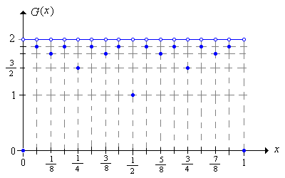
If \(p = \frac{1}{2}\) then \[ G(x) = \begin{cases} 2 - \frac{1}{2^{r(x) - 1}}, & x \text{ is a binary rational} \\ 2, & x \text{ is a binary irrational} \end{cases} \]
Open the bold play experiment. Vary \(x\), \(a\), and \(p\) with the input controls and note how the expected number of trials changes. In particular, note that the mean depends only on the ratio \(x / a\). For selected values of the parameters, run the experiment 1000 times and compare the sample mean to the distribution mean.
For fixed \(x\), \(G\) is continuous as a function of \(p\).
However, as a function of the initial fortune \(x\), for fixed \(p\), the function \(G\) is very irregular.
\(G\) is discontinuous at the binary rationals in \([0, 1]\) and continuous at the binary irrationals.