In this section we will study a family of distributions that has special importance in probability and statistics. In particular, the arrival times in the Poisson process have gamma distributions, and the chi-square distribution in statistics is a special case of the gamma distribution. Also, the gamma distribution is widely used to model physical quantities that take positive values.
Before we can study the gamma distribution, we need to introduce the gamma function, a special function whose values will play the role of the normalizing constants.
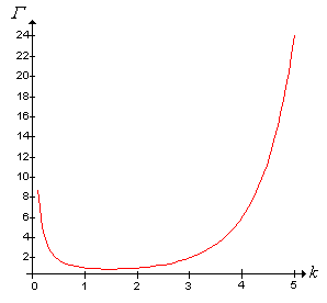
The gamma function \( \Gamma \) is defined as follows \[ \Gamma(k) = \int_0^\infty x^{k-1} e^{-x} \, dx, \quad k \in (0, \infty) \] The function is well defined, that is, the integral converges for any \(k \gt 0\). On the other hand, the integral diverges to \( \infty \) for \( k \le 0 \).
Note that \[ \int_0^\infty x^{k-1} e^{-x} \, dx = \int_0^1 x^{k-1} e^{-x} \, dx + \int_1^\infty x^{k-1} e^{-x} \, dx \] For the first integral on the right, \[\int_0^1 x^{k-1} e^{-x} \, dx \le \int_0^1 x^{k-1} \, dx = \frac{1}{k}\] For the second integral, let \( n = \lceil k \rceil \). Then \[ \int_1^\infty x^{k-1} e^{-x} \, dx \le \int_1^\infty x^{n-1} e^{-x} \, dx \] The last integral can be evaluated explicitly by integrating by parts, and is finite for every \( n \in \N_+ \).
Finally, if \( k \le 0 \), note that \[ \int_0^1 x^{k-1} e^{-x}, \, dx \ge e^{-1} \int_0^1 x^{k-1} \, dx = \infty \]
The gamma function was first introduced by Leonhard Euler.
The (lower) incomplete gamma function is defined by \[ \Gamma(k, x) = \int_0^x t^{k-1} e^{-t} \, dt, \quad k, x \in (0, \infty) \]
Here are a few of the essential properties of the gamma function. The first is the fundamental identity.
\(\Gamma(k + 1) = k \, \Gamma(k)\) for \(k \in (0, \infty)\).
This follows from integrating by parts, with \( u = x^k \) and \( dv = e^{-x} \, dx \): \[ \Gamma(k + 1) = \int_0^\infty x^k e^{-x} \, dx = \left(-x^k e^{-x}\right)_0^\infty + \int_0^\infty k x^{k-1} e^{-x} \, dx = 0 + k \, \Gamma(k) \]
Applying this result repeatedly gives \[ \Gamma(k + n) = k (k + 1) \cdots (k + n - 1) \Gamma(k), \quad n \in \N_+ \] It's clear that the gamma function is a continuous extension of the factorial function.
\(\Gamma(k + 1) = k!\) for \(k \in \N\).
The values of the gamma function for non-integer arguments generally cannot be expressed in simple, closed forms. However, there are exceptions.
\(\Gamma\left(\frac{1}{2}\right) = \sqrt{\pi}\).
By definition, \[ \Gamma\left(\frac{1}{2}\right) = \int_0^\infty x^{-1/2} e^{-x} \, dx \] Substituting \( x = z^2 / 2 \) gives \[ \Gamma\left(\frac{1}{2}\right) = \int_0^\infty \sqrt{2} e^{-z^2/2} \, dz = 2 \sqrt{\pi} \int_0^\infty \frac{1}{\sqrt{2 \pi}} e^{-z^2/2} \, dz\] But the last integrand is the PDF of the standard normal distribution, and so the integral evaluates to \( \frac{1}{2} \)
We can generalize the last result to odd multiples of \( \frac{1}{2} \).
For \( n \in \N \), \[ \Gamma\left(\frac{2 n + 1}{2}\right) = \frac{1 \cdot 3 \cdots (2 n - 1)}{2^n} \sqrt{\pi} = \frac{(2 n)!}{4^n n!} \sqrt{\pi} \]
One of the most famous asymptotic formulas for the gamma function is Stirling's formula, named for James Stirling. First we need to recall a definition.
Suppose that \( f, \, g: D \to (0, \infty) \) where \( D = (0, \infty) \) or \( D = \N_+ \). Then \( f(x) \approx g(x) \) as \( x \to \infty \) means that \[ \frac{f(x)}{g(x)} \to 1 \text{ as } x \to \infty \]
Stirling's formula: \[ \Gamma(x + 1) \approx \left( \frac{x}{e} \right)^x \sqrt{2 \pi x} \text{ as } x \to \infty \]
As a special case of , Stirling's result gives an asymptotic formula for the factorial function: \[ n! \approx \left( \frac{n}{e} \right)^n \sqrt{2 \pi n} \text{ as } n \to \infty \]
The standard gamma distribution with shape parameter \( k \in (0, \infty) \) is a continuous distribution on \( (0, \infty) \) with probability density function \(f\) given by \[ f(x) = \frac{1}{\Gamma(k)} x^{k-1} e^{-x}, \quad x \in (0, \infty) \]
Clearly \( f \) is a valid probability density function, since \( f(x) \gt 0 \) for \( x \gt 0 \), and by definition, \( \Gamma(k) \) is the normalizing constant for the function \( x \mapsto x^{k-1} e^{-x} \) on \( (0, \infty) \).
The following theorem shows that the gamma density has a rich variety of shapes, and shows why \(k\) is called the shape parameter.
The gamma probability density function \( f \) with shape parameter \( k \in (0, \infty) \) satisfies the following properties:
These results follow from standard calculus. For \( x \gt 0 \), \begin{align*} f^\prime(x) &= \frac{1}{\Gamma(k)} x^{k-2} e^{-x}[(k - 1) - x] \\ f^{\prime \prime}(x) &= \frac{1}{\Gamma(k)} x^{k-3} e^{-x} \left[(k - 1)(k - 2) - 2 (k - 1) x + x^2\right] \end{align*}
The special case \(k = 1\) gives the standard exponential distribution. The exponential distribution is studied in more detail in the chapter on Poisson process. When \(k \ge 1\), the gamma distribution is unimodal.
Open the special distribution simulator and select the gamma distribution. Keep the app open as you read this section. First, vary the shape parameter and note the shape of the density function. For various values of \(k\), run the simulation 1000 times and compare the empirical density function to the true probability density function.
The distribution function and the quantile function do not have simple, closed representations for most values of the shape parameter. However, the distribution function has a trivial representation in terms of the incomplete and complete gamma functions in definitions and .
The distribution function \( F \) of the standard gamma distribution with shape parameter \( k \in (0, \infty) \) is given by \[ F(x) = \frac{\Gamma(k, x)}{\Gamma(k)}, \quad x \in (0, \infty) \]
Approximate values of the distribution and quantile functions can be obtained from most mathematical and statistical software packages.
Using the quantile app, find the median, the first and third quartiles, and the interquartile range in each of the following cases:
Suppose that \( X \) has the standard gamma distribution with shape parameter \( k \in (0, \infty) \). The mean and variance are both simply the shape parameter.
The mean and variance of \( X \) are
In the special distribution simulator, select the gamma distribution. Vary the shape parameter and note the size and location of the mean \( \pm \) standard deviation bar. For selected values of \(k\), run the simulation 1000 times and compare the empirical mean and standard deviation to the distribution mean and standard deviation.
More generally, the moments can be expressed easily in terms of the gamma function:
The moments of \( X \) are
Note also that \( \E(X^a) = \infty \) if \( a \le -k \). We can now also compute the skewness and the kurtosis.
The skewness and kurtosis of \( X \) are
In particular, note that \( \skw(X) \to 0 \) and \( \kur(X) \to 3 \) as \( k \to \infty \). Note also that the excess kurtosis \( \kur(X) - 3 \to 0 \) as \( k \to \infty \).
In the special distribution simulator, select the gamma distribution. Increase the shape parameter and note the shape of the density function in light of the previous results on skewness and kurtosis. For various values of \(k\), run the simulation 1000 times and compare the empirical density function to the true probability density function.
Theorem next gives the moment generating function.
The moment generating function of \( X \) is given by \[ \E\left(e^{t X}\right) = \frac{1}{(1 - t)^k}, \quad t \lt 1 \]
For \( t \lt 1 \), \[ \E\left(e^{t X}\right) = \int_0^\infty e^{t x} \frac{1}{\Gamma(k)} x^{k-1} e^{-x} \, dx = \int_0^\infty \frac{1}{\Gamma(k)} x^{k-1} e^{-x(1 - t)} \, dx \] Substituting \( u = x(1 - t) \) so that \( x = u \big/ (1 - t) \) and \( dx = du \big/ (1 - t) \) gives \[ \E\left(e^{t X}\right) = \frac{1}{(1 - t)^k} \int_0^\infty \frac{1}{\Gamma(k)} u^{k-1} e^{-u} \, du = \frac{1}{(1 - t)^k} \]
The gamma distribution is usually generalized by adding a scale parameter. As usual, scale parameters often arise when physical units are changed (inches to centimeters, for example).
If \(Z\) has the standard gamma distribution with shape parameter \(k \in (0, \infty)\) and if \( b \in (0, \infty) \), then \(X = b Z\) has the gamma distribution with shape parameter \(k\) and scale parameter \(b\).
The reciprocal of the scale parameter, \(r = 1 / b\) is known as the rate parameter, particularly in the context of the Poisson process. The gamma distribution with parameters \(k = 1\) and \(b\) is the exponential distribution with scale parameter \(b\) (or rate parameter \(r = 1 / b\)). More generally, when the shape parameter \(k\) is a positive integer, the gamma distribution is known as the Erlang distribution, named for the Danish mathematician Agner Erlang. The exponential distribution governs the time between arrivals in the Poisson model, while the Erlang distribution governs the actual arrival times.
Basic properties of the general gamma distribution follow easily from corresponding properties of the standard distribution and basic results for scale transformations.
Suppose that \( X \) has the gamma distribution with shape parameter \( k \in (0, \infty) \) and scale parameter \( b \in (0, \infty) \).
\(X\) has probability density function \( f \) given by \[ f(x) = \frac{1}{\Gamma(k) b^k} x^{k-1} e^{-x/b}, \quad x \in (0, \infty) \]
Recall that the inclusion of a scale parameter does not change the shape of the density function, but simply scales the graph horizontally and vertically. In particular, we have the same basic shapes as for the standard gamma density function in .
The probability density function \( f \) of \( X \) satisfies the following properties:
In the simulation of the special distribution simulator, select the gamma distribution. Vary the shape and scale parameters and note the shape and location of the probability density function. For various values of the parameters, run the simulation 1000 times and compare the empirical density function to the true probability density function.
Once again, the distribution function and the quantile function do not have simple, closed representations for most values of the shape parameter. However, the distribution function has a simple representation in terms of the incomplete and complete gamma functions in definitions and
The distribution function \( F \) of \( X \) is given by \[ F(x) = \frac{\Gamma(k, x/b)}{\Gamma(k)}, \quad x \in (0, \infty) \]
Approximate values of the distribution and quanitle functions can be obtained from quantile app, and from most mathematical and statistical software packages.
Open the quantile app. Vary the shape and scale parameters and note the shape and location of the distribution and quantile functions. For selected values of the parameters, find the median and the first and third quartiles.
Suppose again that \( X \) has the gamma distribution with shape parameter \( k \in (0, \infty) \) and scale parameter \( b \in (0, \infty) \).
The mean and variance of \( X \) are
In the special distribution simulator, select the gamma distribution. Vary the parameters and note the shape and location of the mean \( \pm \) standard deviation bar. For selected values of the parameters, run the simulation 1000 times and compare the empirical mean and standard deviation to the distribution mean and standard deviation.
The moments of \( X \) are
Note also that \( \E(X^a) = \infty \) if \( a \le -k \). Recall that skewness and kurtosis are defined in terms of the standard score, and hence are unchanged by the addition of a scale parameter.
The skewness and kurtosis of \( X \) are
The moment generating function of \(X\) is given by \[ \E\left(e^{t X}\right) = \frac{1}{(1 - b t)^k}, \quad t \lt \frac{1}{b} \]
Our first result is simply a restatement of the meaning of the term scale parameter.
Suppose that \(X\) has the gamma distribution with shape parameter \(k \in (0, \infty)\) and scale parameter \(b \in (0, \infty)\). If \(c \in (0, \infty)\), then \(c X\) has the gamma distribution with shape parameter \(k\) and scale parameter \(b c\).
More importantly, if the scale parameter is fixed, the gamma family is closed with respect to sums of independent variables.
Suppose that \(X_1\) and \(X_2\) are independent random variables, and that \(X_i\) has the gamma distribution with shape parameter \(k_i \in (0, \infty)\) and scale parameter \(b \in (0, \infty)\) for \(i \in \{1, 2\}\). Then \(X_1 + X_2\) has the gamma distribution with shape parameter \(k_1 + k_2\) and scale parameter \(b\).
Recall that the MGF of \( X = X_1 + X_2 \) is the product of the MGFs of \( X_1 \) and \( X_2 \), so \[ \E\left(e^{t X}\right) = \frac{1}{(1 - b t)^{k_1}} \frac{1}{(1 - b t)^{k_2}} = \frac{1}{(1 - b t)^{k_1 + k_2}}, \quad t \lt \frac{1}{b} \]
From , it follows that the gamma distribution is infinitely divisible:
Suppose that \(X\) has the gamma distribution with shape parameter \(k \in (0, \infty)\) and scale parameter \(b \in (0, \infty)\). For \( n \in \N_+ \), \( X \) has the same distribution as \( \sum_{i=1}^n X_i \), where \((X_1, X_2, \ldots, X_n)\) is a sequence of independent random variables, each with the gamma distribution with with shape parameter \( k / n \) and scale parameter \( b \).
From and the central limit theorm, it follows that if \(k\) is large, the gamma distribution with shape parameter \( k \) and scale parameter \( b \) can be approximated by the normal distribution with mean \(k b\) and variance \(k b^2\). Here is the precise statement:
Suppose that \( X_k \) has the gamma distribution with shape parameter \( k \in (0, \infty) \) and fixed scale parameter \( b \in (0, \infty) \). Then the distribution of the standardized variable below converges to the standard normal distribution as \(k \to \infty\): \[ Z_k = \frac{X_k - k b}{\sqrt{k} b} \]
In the special distribution simulator, select the gamma distribution. For various values of the scale parameter, increase the shape parameter and note the increasingly normal
shape of the density function. For selected values of the parameters, run the experiment 1000 times and compare the empirical density function to the true probability density function.
The gamma distribution is a member of the general exponential family of distributions:
Suppose that \(X\) has gamma distribution with shape parameter \(k \in (0, \infty)\) and scale parameter \(b \in (0, \infty)\). Then the distribution of \(X\) is a two-parameter exponential family with natural parameters \((k - 1, -1 / b)\), and natural statistics \((\ln X, X)\).
This follows from the definition of the general exponential family. The gamma PDF can be written as \[ f(x) = \frac{1}{b^k \Gamma(k)} \exp\left[(k - 1) \ln x - \frac{1}{b} x\right], \quad x \in (0, \infty) \]
For \( n \in (0, \infty) \), the gamma distribution with shape parameter \( n / 2 \) and scale parameter 2 is known as the chi-square distribution with \( n \) degrees of freedom, a distribution that is very important in statistics
Suppose that the lifetime of a device (in hours) has the gamma distribution with shape parameter \(k = 4\) and scale parameter \(b = 100\).
Let \(X\) denote the lifetime in hours.
Suppose that \(Y\) has the gamma distribution with parameters \(k = 10\) and \(b = 2\). For each of the following, compute the true value using the quantile app and then compute the normal approximation. Compare the results.