Earlier, we studied time reversal of discrete-time Markov chains. In continous time, the issues are basically the same. First, the Markov property stated in the form that the past and future are independent given the present, essentially treats the past and future symmetrically. However, there is a lack of symmetry in the fact that in the usual formulation, we have an initial time 0, but not a terminal time. If we introduce a terminal time, then we can run the process backwards in time. In this section, we are interested in the following questions:
Consideration of these questions leads to reversed chains, an important and interesting part of the theory of continuous-time Markov chains. As always, we are also interested in the relationship between properties of a continuous-time chain and the corresponding properties of its discrete-time jump chain. In this section we will see that there are simple and elegant connections between the time reversal of a continuous-time chain and the time-reversal of the jump chain.
Our starting point is a (homogeneous) continuous-time Markov chain \( \bs{X} = \{X_t: t \in [0, \infty)\} \) with (countable ) state space \( S \). We will assume that \( \bs X \) is irreducible, so that every state in \( S \) leads to every other state, and to avoid trivialities, we will assume that there are at least two states. The irreducibility assumption involves no serious loss of generality since otherwise we could simply restrict our attention to an irreducible equivalence class of states. With our usual notation, we will let \( \bs{P} = \{P_t: t \in [0, \infty)\} \) denote the semigroup of transition matrices of \( \bs X \) and \( G \) the infinitesimal generator. Let \( \lambda(x) \) denote the exponential parameter for the holding time in state \( x \in S \) and \( Q \) the transition matrix for the discrete-time jump chain \( \bs{Y} = (Y_0, Y_1, \ldots) \). Finally, let \( \bs U = \{U_\alpha: \alpha \in [0, \infty)\} \) denote the collection of potential matrices of \( \bs X \). We will assume that the chain \( \bs X \) is regular, which gives us the following properties:
The assumption of regularity rules out various types of weird behavior that, while mathematically possible, are usually not appropriate in applications. If \( \bs X \) is uniform, a stronger assumption than regularity, we have the following additional properties:
Now let \( h \in (0, \infty) \). We will think of \( h \) as the terminal time or time horizon so the chains in our first discussion will be defined on the time interval \( [0, h] \). Notationally, we won't bother to indicate the dependence on \( h \), since ultimately the time horizon won't matter. Define \( \hat X_t = X_{h-t} \) for \( t \in [0, h] \). Thus, the process forward in time is \( \bs X = \{X_t: t \in [0, h]\} \) while the process backwards in time is \[ \hat{\bs X} = \{\hat X_t: t \in [0, h]\} = \{X_{h-t}: t \in [0, h]\} \] Similarly let \[\hat{\mathscr F}_t = \sigma\{\hat X_s: s \in [0, t]\} = \sigma\{X_{h-s}: s \in [0, t]\} = \sigma\{X_r: r \in [h - t, h]\}, \quad t \in [0, h]\] So \( \hat{\mathscr{F}}_t \) is the \( \sigma \)-algebra of events of the process \( \hat{\bs X} \) up to time \( t \), which of course, is also the \( \sigma \)-algebra of events of \( \bs X \) from time \( h - t \) forward. Our first result is that the chain reversed in time is still Markov
The process \( \hat{\bs X } = \{\hat X_t: t \in [0, h]\} \) is a Markov chain, but is not time homogeneous in general. For \( s, \, t \in [0, h] \) with \( s \lt t \), the transition matrix from \( s \) to \( t \) is \[ \hat{P}_{s, t}(x, y) = \frac{\P(X_{h - t} = y)}{\P(X_{h - s} = x)} P_{t - s}(y, x), \quad (x, y) \in S^2 \]
Let \( A \in \hat{\mathscr{F}}_s \) and \( x, \, y \in S \). Then \begin{align*} \P(\hat X_t = y \mid \hat X_s = x, A) & = \frac{\P(\hat X_t = y, \hat X_s = x, A)}{\P(\hat X_s = x, A)} = \frac{\P(X_{h - t} = y, X_{h - s} = x, A)}{\P(X_{h - s} = x, A)} \\ & = \frac{\P(A \mid X_{h - t} = y, X_{h - s} = x) \P(X_{h - s} = x \mid X_{h - t} = y) \P(X_{h - t} = y)}{\P(A \mid X_{h - s} = x) \P(X_{h - s} = x)} \end{align*} But \( A \in \sigma\{X_r: r \in [h - s, h]\} \) and \( h - t \lt h - s \), so by the Markov property for \( \bs X \), \[ \P(A \mid X_{h - t} = y, X_{h - s} = x) = \P(A \mid X_{h - s} = x) \] By the time homogeneity of \( \bs X \), \(\P(X_{h - s} = x \mid X_{h - t} = y) = P_{t - s}(y, x)\). Substituting and simplifying gives \[ \P(\hat X_t = y \mid \hat X_s = x, A) = \frac{\P(X_{h - t} = y)}{\P(X_{h - s} = x)} P_{t - s}(y, x) \]
However, the backwards chain will be time homogeneous if \( X_0 \) has an invariant distribution.
Suppose that \( \bs X \) is positive recurrent, with (unique) invariant probability density function \( f \). If \( X_0 \) has the invariant distribution, then \( \hat{\bs X} \) is a time-homogeneous Markov chain. The transition matrix at time \( t \in [0, \infty) \) (for every terminal time \( h \ge t \)), is given by \[ \hat P_t(x, y) = \frac{f(y)}{f(x)} P_t(y, x), \quad (x, y) \in S^2 \]
Exercise holds in the limit of the terminal time, regardless of the initial distribution.
Suppose again that \( \bs X \) is positive recurrent, with (unique) invariant probability density function \( f \). Regardless of the distribution of \( X_0 \), \[\P(\hat X_{s+t} = y \mid \hat X_s = x) \to \frac{f(y)}{f(x)} P_t(y, x) \text{ as } h \to \infty\]
This follows from and our study of the limiting behavior of continuous-time Markov chains. Since \( \bs X \) is irreducible and positive recurrent, \( \P(X_{h - s} = x) \to f(x) \) and \( \P(X_{h - t} = y) \to f(y) \) as \( h \to \infty \) for every \( x, \, y \in S \).
These three results are motivation for the definition that follows. We can generalize by defining the reversal of an irreducible Markov chain, as long as there is a positive, invariant function. Recall that a positive invariant function defines a positive measure on \( S \), but of course not in general a probability measure.
Suppose that \( g: S \to (0, \infty) \) is invariant for \( \bs X \). The reversal of \( \bs X \) with respect to \( g \) is the Markov chain \( \hat{\bs X} = \{\hat X_t: t \in [0, \infty)\} \) with transition semigroup \( \hat{\bs{P}} \) defined by \[\hat P_t (x, y) = \frac{g(y)}{g(x)} P_t(y, x), \quad (x, y) \in S^2, \; t \in [0, \infty)\]
We need to show that the definition makes sense, namely that \( \hat{\bs P} \) defines a transition semigroup for a Markov chain \( \hat{\bs X} \) satisfying the same assumptions that we have imposed on \( \bs X \). First let \( t \in [0, \infty) \). Since \( g \) is invariant for \( \bs X \), \[\sum_{y \in S} \hat P_t(x, y) = \frac{1}{g(x)} \sum_{y \in S} g(y) P_t(y, x) = \frac{g(x)}{g(x)} = 1, \quad x \in S\] Hence \( \hat P_t \) is a valid transition matrix. Next we show that the Chapman-Kolmogorov equations (the semigroup property) holds. Let \( s, \, t \in [0, \infty) \) and \( x, \, z \in S \). Then \begin{align*} \hat P_s \hat P_t (x, z) & = \sum_{y \in S} \hat P_s (x, y) \hat P_t (y, z) = \sum_{y \in S} \frac{g(y)}{g(x)} P_s(y, x) \frac{g(z)}{g(y)} P_t (z, y) \\ & = \frac{g(z)}{g(x)} \sum_{y \in S} P_t(z, y) P_s (y, x) = \frac{g(z)}{g(x)} P_{s+t}(z, x) = \hat P_{s+t}(x, z) \end{align*} Next note that \( \hat P_t(x, x) = P_t(x, x) \) for every \( x \in S \). Hence \( \hat P_t(x, x) \to 1 \) as \( t \downarrow 0 \) for \( x \), so \( \hat{\bs P} \) is also a standard transition semigroup. Note also that if \( \bs P \) is uniform, then so is \( \hat{\bs P} \). Finally, since \( \bs X \) is irreducible, \( P_t(x, y) \gt 0 \) for every \( (x, y) \in S^2 \) and \( t \in (0, \infty) \). Since \( g \) is positive, it follows that \( \hat P_t(y, x) \gt 0 \) for every \( (x, y) \in S^2 \) and \( t \in (0, \infty) \), and hence \( \hat{\bs X} \) is also irreducible.
Recall that if \( g \) is a positive invariant function for \( \bs X \) then so is \( c g \) for every constant \( c \in (0, \infty) \). Note that \( g \) and \( c g \) generate the same reversed chain. So let's consider the cases:
Suppose again that \( \bs X \) is a Markov chain satisfying the assumptions above.
Nonetheless, the general definition is natural, because most of the important properties of the reversed chain follow from the basic balance equation relating the transition semigroups \( \bs{P} \) and \( \hat{\bs{P}} \), and the invariant function \( g \): \[ g(x) \hat P_t(x, y) = g(y) P_t(y, x), \quad (x, y) \in S^2, \; t \in [0, \infty) \] We will see the balance equation repeated for other objects associated with the Markov chains.
Suppose again that \( g: S \to (0, \infty) \) is invariant for \( \bs X \), and that \( \hat{\bs X} \) is the time reversal of \( \bs X \) with respect to \( g \). Then
In the balance equation for the transition semigroups, it's not really necessary to know a-priori that the function \( g \) is invariant, if we know the two transition semigroups.
Suppose that \( g: S \to (0, \infty) \). Then \( g \) is invariant and the Markov chains \( \bs X \) and \( \hat{\bs X} \) are time reversals with respect to \( g \) if and only if \[ g(x) \hat P_t(x, y) = g(y) P_t(y, x), \quad (x, y) \in S^2, \; t \in [0, \infty) \]
All that is left to show is that the balance equation implies that \( g \) is invariant. The computation is exactly the same as in the last result: \[ g P_t(x) = \sum_{y \in S} g(y) P_t(y, x) = \sum_{y \in S} g(x) \hat P_t (x, y) = g(x) \sum_{y \in S} \hat P_t(x, y) = g(x), \quad x \in S \]
Here is a slightly more complicated (but equivalent) version of the balance equation for the transition probabilities.
Suppose again that \( g: S \to (0, \infty) \). Then \( g \) is invariant and the chains \( \bs X \) and \( \hat{\bs X} \) are time reversals with respect to \( g \) if and only if \[ g(x_1) \hat P_{t_1}(x_1, x_2) \hat P_{t_2}(x_2, x_3) \cdots \hat P_{t_n}(x_n, x_{n+1}) = g(x_{n+1}) P_{t_n}(x_{n+1}, x_n) P_{t_{n-1}}(x_n, x_{n-1}) \cdots P_{t_1}(x_2, x_1) \] for all \( n \in \N_+ \), \( (t_1, t_2, \ldots, t_n) \in [0, \infty)^n \), and \( (x_1, x_2, \ldots, x_{n+1}) \in S^{n+1} \).
All that is necessary is to show that the basic balance equation implies the balance equation in the theorem. When \( n = 1 \), we have the basic balance equation itself: \[g(x_1) \hat P_{t_1}(x_1, x_2) = g(x_2) P_{t_1}(x_2, x_1)\] For \( n = 2 \), \[g(x_1) \hat P_{t_1}(x_1, x_2) \hat P_{t_2}(x_2, x_3) = g(x_2)P_{t_1}(x_2, x_1) \hat P_{t_2}(x_2, x_3) = g(x_3)P_{t_2}(x_3, x_2) P_{t_1}(x_2, x_1)\] Continuing in this manner (or using induction) gives the general result.
The balance equation holds for the potenetial matrices.
Suppose again that \( g: S \to (0, \infty) \). Then \( g \) is invariant and the chains \( \bs X \) and \( \hat{\bs X} \) are time reversals with respect to \( g \) if and only if the potential matrices satisfy \[ g(x) \hat U_\alpha(x, y) = g(y) U_\alpha(y, x), \quad (x, y) \in S^2, \; \alpha \in [0, \infty) \]
We just need to show that the balance equation for the transition semigroups is equivalent to the balance equation above for the potential matrices. Suppose first \( g(x) \hat P_t(x, y) = g(y) P_t(y, x) \) for \( t \in [0, \infty) \) and \( (x, y) \in S^2 \). Then \begin{align*} g(x) \hat U_\alpha(x, y) & = g(x) \int_0^\infty e^{-\alpha t} \hat P_t(x, y) dt = \int_0^\infty e^{-\alpha t} g(x) \hat P_t(x, y) dt \\ & = \int_0^\infty e^{-\alpha t} g(y) P_t(y, x) dt = g(y) \int_0^\infty e^{-\alpha t} P_t(y, x) dt = g(y) U_\alpha(y, x) \end{align*} Conversely, suppose that \( g(x) \hat U_\alpha(x, y) = g(y) U_\alpha(y, x) \) for \( (x, y) \in S^2 \) and \( \alpha \in [0, \infty) \). As above, \[ g(x) \hat U_\alpha(x, y) = \int_0^\infty e^{-\alpha t} g(x) \hat P_t(x, y) dt \] So for fixed \( (x, y) \in S^2 \), the function \( \alpha \mapsto g(x) \hat U_\alpha(x, y) \) is the Laplace transform of the time function \( t \mapsto g(x) \hat P_t(x, y) \). Similarly, \( \alpha \mapsto g(y) U_\alpha(x, y) \) is the Laplace transform of the \( t \mapsto g(y) P_t(x, y) \). The Laplace transform of a continuous function uniquely determines the function so it follows that \( g(x) \hat P_t(x, y) = g(y) P_t(y, x) \) for \( t \in [0, \infty) \) and \( (x, y) \in S^2 \).
As a corollary, continuous-time chains that are time reversals are of the same type.
If \( \bs X \) and \( \hat{\bs X} \) are time reversals, then \( \bs X \) and \( \hat{\bs X} \) are of the same type: transient, null recurrent, or positive recurrent.
Suppose that \( \bs X \) and \( \hat{\bs X} \) are time reversals with respect to the invariant function \( g: S \to (0, \infty) \). Then from the previous result, \( \hat U(x, x) = U(x, x) \) for \( x \in S \). The chains are transient if the common potential is finte for each \( x \in S \) and recurrent if the potential is infinite for each \( x \in S \). Suppose that the chains are recurrent. Then \( g \) is unique up to multiplication by positive constants and the chains are both positive recurrent if \( \sum_{x \in S} g(x) \lt \infty \) and both null recurrent if \( \sum_{x \in S} g(x) = \infty \).
The balance equation extends to the infinitesimal generator matrices.
Suppose again that \( g: S \to (0, \infty) \). Then \( g \) is invariant and the Markov chains \( \bs X \) and \( \hat{\bs X} \) are time reversals if and only if the infinitesimal generators satisfy \[ g(x) \hat G(x, y) = g(y) G(y, x), \quad (x, y) \in S^2 \]
We need to show that the balance equation for the transition semigroups is equivalent to the balance equation for the generators. Suppose first that \(g(x) \hat P_t(x, y) = g(y) P_t(y, x)\) for \(t \in [0, \infty)\) and \((x, y) \in S^2\). Taking derivatives with respect to \( t \) and using Kolmogorov's backward equation gives \( g(x) \hat G \hat P_t(x, y) = g(y) G P_t(y, x) \) for \( t \in [0, \infty) \) and \( (x, y) \in S^2\). Evaluating at \( t = 0 \) gives \( g(x) \hat G(x, y) = g(y) G(y, x)\). Conversely, suppose that \(g(x) \hat G(x, y) = g(y) G(y, x)\) for \( (x, y) \in S^2 \). Then repeated application (or induction) shows that \( g(x) \hat G^n(x, y) = g(y) G^n(y, x) \) for every \( n \in \N \) and \((x, y) \in S^2\). If the transition matrices are uniform, we can express them as exponentials of the generators. Hence for \( t \in [0, \infty) \) and \( (x, y) \in S^2 \), \begin{align*} g(x) \hat P_t(x, y) & = g(x) e^{t \hat G(x, y)} = g(x) \sum_{n=0}^\infty \frac{t^n}{n!} \hat G^n(x, y) =\sum_{n=0}^\infty \frac{t^n}{n!} g(x) \hat G^n(x, y)\\ & = \sum_{n=0}^\infty \frac{t^n}{n!} g(y) G^n(y, x) = g(y) \sum_{n=0}^\infty \frac{t^n}{n!} G^n(y, x) = g(y) e^{t G(y, x)} = g(y) P_t(y, x) \end{align*}
This leads to further results and connections:
Suppose again that \( g: S \to (0, \infty) \). Then \( g \) is invariant and \( \bs X \) and \( \hat{\bs X} \) are time reversals with respect to \( g \) if and only if
The exponential parameter functions are related to the generator matrices by \( \lambda(x) = - G(x, x) \) and \( \hat \lambda(x) = -\hat G(x, x) \) for \( x \in S \). The transition matrices for the jump chains are related to the generator matrices by \( Q(x, y) = G(x, y) / \lambda(x) \) and \( \hat Q(x, y) = \hat G(x, y) / \hat \lambda(x) \) for \( (x, y) \in S^2 \) with \( x \ne y \). Hence conditions (a) and (b) are equivalent to \[ g(x) \hat G(x, y) = g(y) G(y, x), \quad (x, y) \in S^2 \] Recall also from the general theory, that if \( g \) is invariant for \( \bs X \) then \( \lambda g \) is invariant for the jump chain \( \bs Y \).
In our original discussion of time reversal in the positive recurrent case, we could have argued that the previous results must be true. If we run the positive recurrent chain \( \bs X = \{X_t: t \in [0, h]\} \) backwards in time to obtain the time reversed chain \( \hat{\bs X} = \{\hat X_t: t \in [0, h]\} \), then the exponential parameters for \( \hat{\bs X} \) must the be same as those for \( \bs X \), and the jump chain \( \hat{\bs Y} \) for \( \hat{\bs X} \) must be the time reversal of the jump chain \( \bs Y \) for \( \bs X \).
Clearly an interesting special case is when the time reversal of a continuous-time Markov chain is stochastically the same as the original chain. Once again, we assume that we have a regular Markov chain \( \bs X = \{X_t: t \in [0, \infty)\} \) that is irreducible on the state space \( S \), with transition semigroup \( \bs P = \{P_t: t \in [0, \infty)\} \). As before, \( \bs U = \{U_\alpha: \alpha \in [0, \infty)\} \) denotes the collection of potential matrices, and \( G \) the infinitesimal generator. Finally, \( \lambda \) denotes the exponential parameter function, \( \bs Y = \{Y_n: n \in \N\} \) the jump chain, and \( Q \) the transition matrix of \( \bs Y \). Here is the definition of reversibility:
Suppose that \( g: S \to (0, \infty) \) is invariant for \( \bs X \). Then \( \bs X \) is reversible with respect to \( g \) if the time reversed chain \( \hat{\bs X} = \{\hat X_t: t \in [0, \infty)\} \) also has transition semigroup \( \bs P \). That is, \[ g(x) P_t(x, y) = g(y) P_t(y, x), \quad (x, y) \in S^2, \; t \in [0, \infty) \]
Clearly if \( \bs X \) is reversible with respect to \( g \) then \( \bs X \) is reversible with respect to \( c g \) for every \( c \in (0, \infty) \). So here is another review of the cases:
Suppose that \( \bs X \) is a Markov chain satisfying the assumptions above.
The following results are corollaries of the results above for time reversals. First, we don't need to know a priori that the function \( g \) is invariant.
Suppose that \( g: S \to (0, \infty) \). Then \( g \) is invariant and \( \bs X \) is reversible with respect to \( g \) if and only if \[ g(x) P_t(x, y) = g(y) P_t(y, x), \quad (x, y) \in S^2, \; t \in [0, \infty) \]
Suppose again that \( g: S \to (0, \infty) \). Then \( g \) is invariant and \( \bs X \) is reversible with respect to \( g \) if and only if \[ g(x_1) P_{t_1}(x_1, x_2) P_{t_2}(x_2, x_3) \cdots P_{t_n}(x_n, x_{n+1}) = g(x_{n+1}) P_{t_n}(x_{n+1}, x_n) P_{t_{n-1}}(x_n, x_{n-1}) \cdots P_{t_1}(x_2, x_1) \] for all \( n \in \N_+ \), \( (t_1, t_2, \ldots, t_n) \in [0, \infty)^n \), and \( (x_1, x_2, \ldots, x_{n+1}) \in S^{n+1} \).
Suppose again that \( g: S \to (0, \infty) \). Then \( g \) is invariant and \( \bs X \) is reversible with respect to \( g \) if and only if \[ g(x) U_\alpha(x, y) = g(y) U_\alpha(y, x), \quad (x, y) \in S^2, \; \alpha \in [0, \infty) \]
Suppose again that \( g: S \to (0, \infty) \). Then \( g \) is invariant and \( \bs X \) is reversible with respect to \( g \) if and only if \[ g(x) G(x, y) = g(y) G(y, x), \quad (x, y) \in S^2 \]
Suppose again that \( g: S \to (0, \infty) \). Then \( g \) is invariant and \( \bs X \) is reversible if and only if the jump chain \( \bs Y \) is reversible with respect to \( \lambda g \).
Recall that \( \bs X \) is recurrent if and only if the jump chain \( \bs Y \) is recurrent. In this case, the invariant functions for \( \bs X \) and \( \bs Y \) exist and are unique up to positive constants. So in this case, the previous theorem states that \( \bs X \) is reversible if and only if \( \bs Y \) is reversible. In the positive recurrent case (the most important case), the following theorem gives a condition for reversibility that does not directly reference the invariant distribution. The condition is known as the Kolmogorov cycle condition, and is named for Andrei Kolmogorov
Suppose that \( \bs X \) is positive recurrent. Then \( \bs X \) is reversible if and only if for every sequence of distinct states \( (x_1, x_2, \ldots, x_n) \), \[ G(x_1, x_2) G(x_2, x_3) \cdots G(x_{n-1}, x_n) G(x_n, x_1) = G(x_1, x_n) G(x_n, x_{n-1}) \cdots G(x_3, x_2) G(x_2, x_1) \]
Suppose that \( \bs X \) is reversible, and let \( f \) denote the invariant PDF of \( \bs X \). Then \( G(x, y) = \frac{f(y)}{f(x)} G(x, y) \) for \( (x, y) \in S^2 \). Substituting gives the Kolmogorov cycle condition. Conversely, suppose that the Kolmogorov cycle condition holds for \( \bs X \). Recall that \( G(x, y) = \lambda(x) Q(x, y) \) for \( (x, y) \in S^2 \). Substituting into the cycle condition for \( \bs X \) gives the cycle condition for \( \bs Y \). Hence \( \bs Y \) is reversible and therefore so is \( \bs X \).
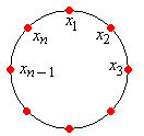
Note that the Kolmogorov cycle condition states that the transition rate of visiting states \( (x_2, x_3, \ldots, x_n, x_1) \) in sequence, starting in state \( x_1 \) is the same as the transition rate of visiting states \( (x_n, x_{n-1}, \ldots, x_2, x_1) \) in sequence, starting in state \( x_1 \). The cycle condition is also known as the balance equation for cycles.
The continuous-time, two-state chain has been studied in our previous sections on continuous-time chains, so naturally we are interested in time reversal.
Consider the continuous-time Markov chain \( \bs{X} = \{X_t: t \in [0, \infty)\} \) on \( S = \{0, 1\} \) with transition rate \( a \in (0, \infty) \) from 0 to 1 and transition rate \( b \in (0, \infty) \) from 1 to 0. Show that \( \bs X \) is reversible
First note that \( \bs X \) is irreducible since \( a \gt 0 \) and \( b \gt 0 \). Since \( S \) is finite, \( \bs X \) is positive recurrent.
Of course, the invariant PDF \( f \) is \( f(0) = b / (a + b) \), \( f(1) = a / (a + b) \).
The Markov chain in the following exercise has also been studied in previous sections.
Consider the Markov chain \( \bs X = \{X_t: t \in [0, \infty)\} \) on \( S = \{0, 1, 2\} \) with exponential parameter function \( \lambda = (4, 1, 3) \) and jump transition matrix \[ Q = \left[\begin{matrix} 0 & \frac{1}{2} & \frac{1}{2} \\ 1 & 0 & 0 \\ \frac{1}{3} & \frac{2}{3} & 0\end{matrix}\right] \] Give each of the following for the time reversed chain \( \hat{\bs X} \):
Note that the chain is irreducible, and since \( S \) is finite, positive recurrent. We found previously that an invariant function (unique up to multiplication by positive constants) is \( g = (3, 10, 2) \).
Time reversal is discussed for the following special models in spearate sections.