Most of the important topological spaces that occur in applications (like probability) have an additional structure that gives a distance between points in the space.
A metric space \((S, d)\) consists of a nonempty set \( S \) and a function \( d: S \times S \to [0, \infty) \) that satisfies the following axioms: For \( x, \, y, \, z \in S \),
The function \( d \) is known as a metric or a distance function.
So as the name suggests, \( d(x, y) \) is the distance between points \( x, \, y \in S \). The axioms are intended to capture the essential properties of distance from geometry. Part (a) is the positive property; the distance is strictly positive if and only if the points are distinct. Part (b) is the symmetric property; the distance from \( x \) to \( y \) is the same as the distance from \( y \) to \( x \). Part (c) is the triangle inequality; going from \( x \) to \( z \) cannot be longer than going from \( x \) to \( z \) by way of a third point \( y \).
Note that if \( (S, d) \) is a metric space, and \( A \) is a nonempty subset of \( S \), then the set \( A \) with \( d \) restricted to \( A \times A \) is also a metric space (known as a subspace). The next definitions also come naturally from geometry:
Suppose that \( (S, d) \) is a metric space, and that \( x \in S \) and \( r \in (0, \infty) \).
A metric on a space induces a topology on the space in a natural way.
Suppose that \( (S, d) \) is a metric space. By definition, a set \( U \subseteq S \) is open if for every \( x \in U \) there exists \( r \in (0, \infty) \) such that \( B(x, r) \subseteq U \). The collection \( \ms S_d \) of open subsets of \( S \) is a topology.
As the names suggests, an open ball is in fact open and a closed ball is in fact closed.
Suppose again that \( (S, d) \) is a metric space, and that \( x \in S \) and \( r \in (0, \infty) \). Then
Recall that for a general topological space, a neighborhood of a point \( x \in S \) is a set \( A \subseteq S \) with the property that there exists an open set \( U \) with \( x \in U \subseteq A \). It follows that in a metric space, \( A \subseteq S \) is a neighborhood of \( x \) if and only if there exists \( r \gt 0 \) such that \( B(x, r) \subseteq A \). In words, a neighborhood of a point must contain an open ball about that point.
It's easy to construct new metrics from ones that we already have. Here's one such result.
Suppose that \( S \) is a nonempty set, and that \( d, \, e \) are metrics on \( S \), and \( c \in (0, \infty) \). Then the following are also metrics on \( S \):
Since a metric space produces a topological space, all of the definitions for general topological spaces apply to metric spaces as well. In particular, in a metric space, distinct points can always be separated.
A metric space \( (S, d) \) is a Hausdorff space.
Let \( x, \, y \) be distinct points in \( S \). Then \(r = d(x, y) \gt 0\). The sets \( B(x, r/2) \) and \( B(y, r/2) \) are open, and contain \( x \) and \( y \), respectively. Suppose that \( z \in B(x, r/2) \cap B(y, r/2) \). By the triangle inequality, \[ d(x, y) \le d(x, z) + d(z, y) \lt \frac{r}{2} + \frac{r}{2} = r \] a contradiction. Hence \( B(x, r/2) \) and \( B(y, r/2) \) are disjoint.
Again, every metric space is a topological space, but not conversely. A non-Hausdorff space, for example, cannot correspond to a metric space. We know there are such spaces: a set \( S \) with more than one point, and with the trivial topology \( \ms S = \{S, \emptyset\} \) is non-Hausdorff.
Suppose that \( (S, \ms S) \) is a topological space. If there exists a metric \( d \) on \( S \) such that \( \ms S = \ms S_d \), then \( (S, \ms S) \) is said to be metrizable.
It's easy to see that different metrics can induce the same topology. For example, if \( d \) is a metric and \( c \in (0, \infty) \), then the metrics \( d \) and \( c d \) induce the same topology.
Let \( S \) be a nonempty set. Metrics \( d \) and \( e \) on \(S\) are equivalent, and we write \( d \equiv e \), if \( \ms S_d = \ms S_e \). The relation \( \equiv \) is an equivalence realation on the collection of metrics on \( S \). That is, for metrics \( d, \, e, \, f \) on \( S \),
There is a simple condition that characterizes when the topology of one metric is finer than the topology of another metric, and then this in turn leads to a condition for equivalence of metrics.
Suppose again that \( S \) is a nonempty set and that \( d, \, e \) are metrics on \( S \). Then \( \ms S_e \) is finer than \( \ms S_d \) if and only if every open ball relative to \( d \) contains an open ball relative to \( e \).
Suppose that \( \ms S_d \subseteq \ms S_e \) so that \( \ms S_e \) is finer than \( \ms S_d \). If \( x \in S \) and \( a \in (0, \infty) \), then the open ball \( B_d(x, a) \) centered at \( x \) of radius \( a \) for the metric \( d \) is in \( \ms S_d \) and hence in \( \ms S_e \). Thus there exists \( b \in (0, \infty) \) such that \( B_e(x, b) \subseteq B_d(x, a) \). Conversely, suppose that the condition in the theorem holds and suppose that \( U \in \ms S_d \). If \( x \in U \) there exists \( a \in (0, \infty) \) such that \( B_d(x, a) \subseteq U \). Hence there exists \( b \in (0, \infty) \) such that \( B_e(x, b) \subseteq B_d(x, a) \subseteq U \). So \( U \in \ms S_e \).
It follows that metrics \( d \) and \( e \) on \( S \) are equivalent if and only if every open ball relative to one of the metrics contains an open ball relative to the other metric.
So every metrizable topology on \( S \) corresponds to an equivalence class of metrics that produce that topology. Sometimes we want to know that a topological space is metrizable, because of the nice properties that it will have, but we don't really need to use a specific metric that generates the topology. At any rate, it's important to have conditions that are sufficient for a topological space to be metrizable. The most famous such result is the Urysohn metrization theorem, named for the Russian mathematician Pavel Uryshon:
Suppose that \( (S, \ms S) \) is a regular, second-countable, Hausdorff space. Then \( (S, \ms S) \) is metrizable.
Recall that regular means that every closed set and point not in the set can be separated by disjoint open sets. As discussed earlier, Hausdorff means that any two distinct points can be separated by disjoint open sets. Finally, second-countable means that there is a countable base for the topology, that is, there is a countable collection of open sets with the property that every other open set is a union of sets in the collection.
With a distance function, the convergence of a sequence can be characterized in a manner that is just like calculus. Recall that for a general topological space \( (S, \ms S) \), if \( (x_n: n \in \N_+) \) is a sequence of points in \( S \) and \( x \in S \), then \( x_n \to x \) as \( n \to \infty \) means that for every neighborhood \( U \) of \( x \), there exists \( m \in \N_+ \) such that \( x_n \in U \) for \( n \gt m \).
Suppose that \( (S, d) \) is a metric space, and that \( (x_n: n \in \N_+) \) is a sequence of points in \( S \) and \( x \in S \). Then \( x_n \to x \) as \( n \to \infty \) if and only if for every \( \epsilon \gt 0 \) there exists \( m \in \N_+ \) such that if \( n \gt m \) then \( d(x_n, x) \lt \epsilon \). Equivalently, \( x_n \to x \) as \( n \to \infty \) if and only if \( d(x_n, x) \to 0 \) as \( n \to \infty \) (in the usual calculus sense).
Suppose that \( x_n \to x \) as \( n \to \infty \), and let \( \epsilon \gt 0 \). Then \( B(x, \epsilon) \) is a neighborhood of \( x \), so there exists \( m \in \N_+ \) such that \( x_n \in B(x, \epsilon) \) for \( n \gt m \), which is the condition in the theorem. Conversely, suppose that condition in the theorem holds, and let \( U \) be a neighborhood of \( x \). Then there exists \( \epsilon \gt 0 \) such that \( B(x, \epsilon) \subseteq U \). By assumption, there exists \( m \in \N_+ \) such that if \( n \gt m \) then \( x_n \in B(x, \epsilon) \subseteq U \).
So, no matter how tiny \( \epsilon \gt 0 \) may be, all but finitely many terms of the sequence are within \( \epsilon \) distance of \( x \). As one might hope, limits are unique.
Suppose again that \( (S, d) \) is a metric space. Suppose also that \( (x_n: n \in \N_+) \) is a sequence of points in \( S \) and that \( x, \, y \in S \). If \( x_n \to x \) as \( n \to \infty \) and \( x_n \to y \) as \( n \to \infty \) then \( x = y \).
This follows immediately since a metric space is a Hausdorff space, and the limit of a sequence in a Hausdorff space is unique. Here's a direct proof: Let \( \epsilon \gt 0 \). Then there exists \( k \in \N_+ \) such that \( d(x_n, x) \lt \epsilon / 2 \) for \( n \gt k \), and there exists \( m \in \N_+ \) such that \( d(x_n, y) \lt \epsilon / 2 \) for \( n \gt m \). Let \( n \gt \max\{k, m\} \). By the triangle inequality, \[ d(x, y) \le d(x, x_n) + d(x_n, y) \lt \frac{\epsilon}{2} + \frac{\epsilon}{2} = \epsilon \] So we have \( d(x, y) \lt \epsilon \) for every \( \epsilon \gt 0 \) and hence \( d(x, y) = 0 \) and thus \( x = y \).
Convergence of a sequence is a topological property, and so is preserved under equivalence of metrics.
Suppose that \( d, \, e \) are equivalent metrics on \( S \), and that \( (x_n: n \in \N_+) \) is a sequence of points in \( S \) and \( x \in S \). Then \( x_n \to x \) as \( n \to \infty \) relative to \( d \) if and only if \( x_n \to x \) as \( n \to \infty \) relative to \( e \).
Closed subsets of a metric space have a simple characterization in terms of convergent sequences, and this characterization is more intuitive than the abstract axioms in a general topological space.
Suppose again that \( (S, d) \) is a metric space. Then \( A \subseteq S \) is closed if and only if whenever a sequence of points in \( A \) converges, the limit is also in \( A \).
Suppose that \( A \) is closed and that \( (x_n: n \in \N_+) \) is a sequence of points in \( A \) with \( x_n \to x \in S \) as \( n \to \infty \). Suppose that \( x \in A^c \). Since \( A^c \) is open, \( x_n \in A^c \) for \( n \) sufficiently large, a contradiction. Hence \( x \in A \). Conversely, suppose that \( A \) has the sequential closure property, but that \( A \) is not closed. Then \( A^c \) is not open. This means that there exists \( x \in A^c \) with the property that every neighborhood of \( x \) has points in \( A \). Specifically, for each \( n \in \N_+ \) there exists \( x_n \in B(x, 1/n) \) with \( x_n \in A \). But clearly \( x_n \to x \) as \( n \to \infty \), again a contradiction.
The following definition also shows up in standard calculus. The idea is to have a criterion for convergence of a sequence that does not require knowing a-priori the limit. But for metric spaces, this definition takes on added importance.
Suppose again that \( (S, d) \) is a metric space. A sequence of points \( (x_n: n \in \N_+) \) in \( S \) is a Cauchy sequence if for every \( \epsilon \gt 0 \) there exist \( k \in \N_+ \) such that if \( m, \, n \in \N_+ \) with \( m \gt k \) and \( n \gt k \) then \( d(x_m, x_n) \lt \epsilon \).
Cauchy sequences are named for the ubiquitous Augustin Cauchy. So for a Cauchy sequence, no matter how tiny \( \epsilon \gt 0 \) may be, all but finitely many terms of the sequence will be within \( \epsilon \) distance of each other. A convergent sequence is always Cauchy.
Suppose again that \( (S, d) \) is a metric space. If a sequence of points \( (x_n: n \in \N_+) \) in \( S \) converges, then the sequence is Cauchy.
By assumption, there exists \( x \in S \) such that \( x_n \to x \) as \( n \to \infty \). Let \( \epsilon \gt 0 \). There exists \( k \in \N_+ \) such that if \( n \in \N_+ \) and \( n \gt k \) then \( d(x_n, x) \lt \epsilon / 2 \). Hence if \( m, \, n \in \N_+ \) with \( m \gt k \) and \( n \gt k \) then by the triangle inequality, \[ d(x_m, x_n) \le d(x_m, x) + d(x, x_n) \lt \frac{\epsilon}{2} + \frac{\epsilon}{2} = \epsilon \] So the sequence is Cauchy.
Conversely, one might think that a Cauchy sequence should converge, but it's relatively trivial to create a situation where this is false. Suppose that \( (S, d) \) is a metric space, and that there is a point \( x \in S \) that is the limit of a sequence of points in \( S \) that are all distinct from \( x \). Then the space \( T = S - \{x\} \) with the metric \( d \) restricted to \( T \times T \) has a Cauchy sequence that does not converge. Essentially, we have created a convergence hole
. So our next defintion is very natural and very important.
Suppose again that \( (S, d) \) is metric space and that \( A \subseteq S \). Then \( A \) is complete if every Cauchy sequence in \( A \) converges to a point in \( A \).
Of course, completeness can be applied to the entire space \( S \). Trivially, a complete set must be closed.
Suppose again that \( (S, d) \) is a metric space, and that \( A \subseteq S \). If \( A \) is complete, then \( A \) is closed.
Completeness is such a crucial property that it is often imposed as an assumption on metric spaces that occur in applications. Even though a Cauchy sequence may not converge, here is a partial result that will be useful latter: if a Cauchy sequence has a convergent subsequence, then the sequence itself converges.
Suppose again the \( (S, d) \) is a metric space, and that \( (x_n: n \in \N_+) \) is a Cauchy sequence in \( S \). If there exists a subsequence \( \left(x_{n_k}: k \in \N_+\right) \) such that \( x_{n_k} \to x \in S \) as \( k \to \infty \), then \( x_n \to x \) as \( n \to \infty \).
Recall that in the construction of a subsequence, the indices \( (n_k: k \in \N_+) \) must be a strictly increasing sequence in \( \N_+ \). In particular, \( n_k \to \infty \) as \( k \to \infty \). So let \( \epsilon \gt 0 \). From the hypotheses, there exists \( j \in \N_+ \) such that if \( k \gt j \) then \( d\left(x_{n_k}, x\right) \lt \epsilon / 2 \). There exists \( N \in \N_+ \) such that if \( m \gt N \) and \( p \gt N \) then \( d(x_m, x_p) \lt \epsilon / 2 \). Now let \( m \gt N \). Pick \( k \in \N_+ \) such that \( k \gt j \) and \( n_k \gt N \). By the triangle inequality, \[ d(x_m, x) \le d\left(x_m, x_{n_k}\right) + d\left(x_{n_k}, x\right) \le \frac{\epsilon}{2} + \frac{\epsilon}{2} = \epsilon \]
In metric spaces, continuity of functions also has simple characterizations in terms that are familiar from calculus. We start with local continuity. Recall that the general topological definition is that \( f: S \to T \) is continuous at \( x \in S \) if \( f^{-1}(V) \) is a neighborhood of \( x \) in \( S \) for every open neighborhood \( V \) of \( f(x) \) in \( T \).
Suppose that \( (S, d) \) and \( (T, e) \) are metric spaces, and that \( f: S \to T \). The continuity of \( f \) at \( x \in S \) is equivalent to each of the following conditions:
More generally, recall that \( f \) continuous on \( A \subseteq S \) means that \( f \) is continuous at each \( x \in A \), and that \( f \) continuous means that \( f \) is continuous on \(S \). So general continuity can be characterized in terms of sequential continuity and the \( \epsilon \)-\( \delta \) condition. But on a metric space, there are stronger versions of continuity.
Suppose again that \( (S, d) \) and \( (T, e) \) are metric spaces and that \( f: S \to T \). Then \( f \) is uniformly continuous if for every \( \epsilon \gt 0 \) there exists \( \delta \gt 0 \) such that if \( x, \, y \in S \) with \( d(x, y) \lt \delta \) then \( e[f(x), f(y)] \le \epsilon \).
In the \(\epsilon\)-\( \delta \) formulation of ordinary point-wise continuity above, \( \delta \) depends on the point \( x \) in addition to \( \epsilon \). With uniform continuity, there exists a \( \delta \) depending only on \( \epsilon \) that works uniformly in \( x \in S \).
Suppose again that \( (S, d) \) and \( (T, e) \) are metric spaces, and that \( f: S \to T \). If \( f \) is uniformly continuous then \( f \) is continuous.
Here is an even stronger version of continuity.
Suppose again that \( (S, d) \) and \( (T, e) \) are metric spaces, and that \( f: S \to T \). Then \( f \) is Höder continuous with exponent \( \alpha \in (0, \infty) \) if there exists \( C \in (0, \infty) \) such that \( e[f(x), f(y)] \le C [d(x, y)]^\alpha \) for all \( x, \, y \in S \).
The definition is named for Otto Höder. The exponent \( \alpha \) is more important than the constant \( C \), which generally does not have a name. If \( \alpha = 1 \), \( f \) is said to be Lipschitz continuous, named for the German mathematician Rudolf Lipschitz.
Suppose again that \( (S, d) \) and \( (T, e) \) are metric spaces, and that \( f: S \to T \). If \( f \) is Höder continuous with exponent \( \alpha \gt 0 \) then \( f \) is uniformly continuous.
The case where \( \alpha = 1 \) and \( C \lt 1 \) is particularly important.
Suppose again that \( (S, d) \) and \( (T, e) \) are metric spaces. A function \( f: S \to T \) is a contraction if there exists \( C \in (0, 1) \) such that \[ e[f(x), f(y)] \le C d(x, y), \quad x, \, y \in S \]
So contractions shrink distance. By , a contraction is uniformly continuous. Part of the importance of contraction maps is due to the famous Banach fixed-point theorem, named for Stefan Banach.
Suppose that \( (S, d) \) is a complete metric space and that \( f: S \to S \) is a contraction. Then \( f \) has a unique fixed point. That is, there exists exactly one \( x^* \in S \) with \( f(x^*) = x^* \). Let \( x_0 \in S \), and recursively define \( x_n = f(x_{n-1}) \) for \( n \in \N_+ \). Then \( x_n \to x^* \) as \( n \to \infty \).
Functions that preserve distance are particularly important. The term isometry means distance-preserving.
Suppose again that \( (S, d) \) and \( (T, e) \) are metric spaces, and that \( f: S \to T \). Then \( f \) is an isometry if \( e[f(x), f(y)] = d(x, y) \) for every \( x, \, y \in S \).
Suppose again that \( (S, d) \) and \( (T, e) \) are metric spaces, and that \( f: S \to T \). If \( f \) is an isometry, then \( f \) is one-to-one and Lipschitz continuous.
In particular, an isometry \( f \) is uniformly continuous, again by . If one metric space can be mapped isometrically onto another metric space, the spaces are essentially the same.
Metric spaces \( (S, d) \) and \( (T, e) \) are isometric if there exists an isometry \( f \) that maps \( S \) onto \( T \). Isometry is an equivalence relation on metric spaces. That is, for metric spaces \( (S, d) \), \( (T, e) \), and \( (U, \rho) \),
In particular, if metric spaces \( (S, d) \) and \( (T, e) \) are isometric, then as topological spaces, they are homeomorphic.
In a metric space, various definitions related to a set being bounded are natural, and are related to the general concept of compactness.
Suppose again that \( (S, d) \) is a metric space, and that \( A \subseteq S \). Then \( A \) is bounded if there exists \( r \in (0, \infty) \) such that \( d(x, y) \le r \) for all \( x, \, y \in A \). The diameter of \( A \) is \[ \diam(A) = \inf\{r \gt 0: d(x, y) \lt r \text{ for all } x, \, y \in A\} \]
Recall that \( \inf(\emptyset) = \infty \), so \(\diam(A) = \infty \) if \( A \) is unbounded. In the bounded case, note that if the distance between points in \( A \) is bounded by \( r \in (0, \infty) \), then the distance is bounded by any \( s \in [r, \infty) \). Hence the diameter definition makes sense.
So \( A \) is bounded if and only if \( \diam(A) \lt \infty \). Diameter is an increasing function relative to the subset partial order.
Suppose again that \( (S, d) \) is a metric space, and that \( A \subseteq B \subseteq S \). Then \( \diam(A) \le \diam(B) \).
Our next definition is stronger, but first let's review some terminology that we used for general topological spaces: If \( S \) is a set, \( A \) a subset of \( S \), and \( \ms A \) a collection of subsets of \( S \), then \( \ms A \) is said to cover \( A \) if \( A \subseteq \bigcup \ms A \). So with this terminology, we can talk about open covers, closed covers, finite covers, disjoint covers, and so on.
Suppose again that \( (S, d) \) is a metric space, and that \( A \subseteq S \). Then \( A \) is totally bounded if for every \( r \gt 0 \) there is a finite cover of \( A \) with open balls of radius \( r \).
Recall that for a general topological space, a set \( A \) is compact if every open cover of \( A \) has a finite subcover. So in a metric space, the term precompact is sometimes used instead of totally bounded: The set \( A \) is totally bounded if every cover of \( A \) with open balls of radius \( r \) has a finite subcover.
Suppose again that \( (S, d) \) is a metric space. If \( A \subseteq S \) is totally bounded then \( A \) is bounded.
There exists a finite cover of \( A \) with open balls of radius 1. Let \( C \) denote the set of centers of the balls, and let \( c = \max\{d(u, v): u, \, v \in C\} \), the maximum distance between two centers. Since \( C \) is finite, \( c \lt \infty \). Now let \( x, \, y \in A \). Since the balls cover \( A \), there exist \( u, \, v \in C \) with \( x \in B(u, 1) \) and \( y \in B(v, 1) \). By the triangle inequality (what else?) \[ d(x, y) \le d(x, u) + d(u, v) + d(v, y) \le 2 + c \] Hence \( A \) is bounded.
Since a metric space is a Hausdorff space, a compact subset of a metric space is closed. Compactness also has a simple characterization in terms of convergence of sequences.
Suppose again that \( (S, d) \) is a metric space. A subset \( C \subseteq S \) is compact if and only if every sequence of points in \( C \) has a subsequence that converges to a point in \( C \).
The condition in the theorem is known as sequential compactness, so we want to show that sequential compactness is equivalent to compactness. The proof is harder than most of the others in this section, but the proof presented here is the nicest I have found, and is due to Anton Schep.
Suppose that \( C \) is compact and that \( \bs x = (x_n: n \in \N_+) \) is a sequence of points in \( C \). Let \( A = \{x_n: n \in \N_+\} \subseteq C\), the unordered set of distinct points in the sequence. If \( A \) is finite, then some element of \( a \in A \) must occur infinitely many times in the sequence. In this case, we can construct a subsequence of \( \bs x \) all of whose terms are \( a \), and so this subsequence trivially converges to \( a \in C \). Suppose next that \( A \) is infinite. Since the space is Hausdorff, \( C \) is closed, and therefore \( \cl(A) \subseteq C \). Our next claim is that there exists \( a \in \cl(A) \) such that for every \( r \gt 0 \), the set \( A \cap B(a, r) \) is infinte. If the claim is false, then for each \( a \in \cl(A) \) there exists \( r_a \gt 0 \) such that \( A \cap B(a, r) \) is finite. It then follows that for each \( a \in A \), there exists \( \epsilon_a \gt 0 \) such that \( A \cap B(a, \epsilon_a) = \{a\} \). But then \( \ms{U} = \{B(a, \epsilon_a): a \in \cl(A)\} \cup \{[\cl(A)]^c\} \) is an open cover of \( C \) that has no finite subcover, a contradiction. So the claim is true and for some \( a \in \cl(A) \), the set \( A \cap B(a, r) \) is infinite for each \( r \gt 0 \). We can construct a subsequence of \( \bs x \) that converges to \( a \in C \).
Conversely, suppose that \( C \) is sequentially compact. If \( \bs x = (x_n: n \in \N_+) \) is a Cauchy sequence in \( C \), then by assumption, \( \bs x \) has a subsequence that converges to some \( x \in C \). But then by the sequence \( \bs x \) itself converges to \( x \), so it follows that \( C \) is complete. We next show that \( C \) is totally bounded. Our goal is to show that \( C \) can be covered by a finite number of balls of an arbitrary radius \( r \gt 0 \). Pick \( x_1 \in C \). If \( C \subseteq B(x_1, r) \) then we are done. Otherwise, pick \( x_2 \in C \setminus B(x_1, r) \). If \( C \subseteq B(x_1, r) \cup B(x_2, r) \) then again we are done. Otherwise there exists \( x_3 \in C \setminus [B(x_1, r) \cup B(x_2, r)] \). This process must terminate in a finite number of steps or otherwise we would have a sequence of points \( (x_n: n \in \N_+) \) in \( C \) with the property that \( d(x_n, x_m) \ge r \) for every \( n, \, m \in \N_+ \). Such a sequence does not have a convergent subsequence. Suppose now that \( \ms{U} \) is an open cover of \( C \) and let \( c = \diam(C) \). Then \( C \) can be covered by a finite number of closed balls of with centers in \( C \) and with radius \( c / 4 \). It follows that at least one of these balls cannot be covered by a finite subcover from \( \ms{U} \). Let \( C_1 \) denote the intersection of this ball with \( C \). Then \( C_1 \) is closed and is sequentially compact with \( \diam(C_1) \le c / 4 \). Repeating the argument, we generate a nested sequence of close sets \( (C_1, C_2, \ldots) \) such that \( \diam(C_n) \le c / 2^n \), and with the property that \( C_n \) cannot be finitely covered by \( \ms{U} \) for each \( n \in \N_+ \). Pick \( x_n \in C_n \) for each \( n \in \N_+ \). Then \( \bs x = (x_n: n \in \N_+) \) is a Cauchy sequence in \( C \) and hence has a subsequence that converges to some \( x \in C \). Then \( x \in \bigcap_{n=1}^\infty C_n \) and since \( \diam(C_n) \to 0 \) as \( n \to \infty \) it follows that in fact, \( \bigcap_{n=1}^\infty C_n = \{x\}\). Now, since \( \ms{U} \) covers \( C \), there exists \( U \in \ms{U} \) such that \( x \in U \). Since \( U \) is open, there exists \( r \gt 0 \) such that \( B(x, r) \subseteq U \). Now let \( n \in \N_+ \) be sufficiently large that \( d(x, x_n) \le r / 2 \) and \( \diam(C_n) \lt r / 2 \). Then \( C_n \subseteq B(x, r) \subseteq U \), which contradicts the fact that \( C_n \) cannot be finitely covered by \( \ms{U} \).
Our last discussion is somewhat advanced, but is important for the study of certain random processes, particularly Brownian motion. The idea is to measure the size
of a set in a metric space in a topological way, and then use this measure to define a type of dimension
. We need a preliminary definition, using our convenient cover terminology. If \( (S, d) \) is a metric space, \( A \subseteq S \), and \( \delta \in (0, \infty) \), then a countable \( \delta \) cover of \( A \) is a countable cover \( \ms B \) of \( A \) with the property that \( \diam(B) \lt \delta \) for each \( B \in \ms B \).
Suppose again that \( (S, d) \) is a metric space and that \( A \subseteq S \). For \( \delta \in (0, \infty) \) and \( k \in [0, \infty) \), define \[ H_\delta^k(A) = \inf\left\{\sum_{B \in \ms B} \left[\diam(B)\right]^k: \ms B \text{ is a countable } \delta \text{ cover of } A \right\} \] The \( k \)-dimensional Hausdorff measure of \( A \) is \[ H^k(A) = \sup \left\{H_\delta^k(A): \delta \gt 0\right\} = \lim_{\delta \downarrow 0} H_\delta^k(A) \]
Note that if \( \ms B \) is a countable \( \delta \) cover of \( A \) then it is also a countable \( \epsilon \) cover of \( A \) for every \( \epsilon \gt \delta \). This means that \( H_\delta^k(A) \) is decreasing in \( \delta \in (0, \infty) \) for fixed \( k \in [0, \infty) \). Hence \[ \sup \left\{H_\delta^k(A): \delta \gt 0\right\} = \lim_{\delta \downarrow 0} H_\delta^k(A) \]
Note that the \( k \)-dimensional Hausdorff measure is defined for every \( k \in [0, \infty) \), not just nonnegative integers. Nonetheless, the integer dimensions are interesting. The 0-dimensional measure of \( A \) is the number of points in \( A \). In Euclidean space, which we consider below in , the measures of dimension 1, 2, and 3 are related to length, area, and volume, respectively.
Suppose again that \( (S, d) \) is a metric space and that \( A \subseteq S \). The Hausdorff dimension of \( A \) is \[ \dim_H(A) = \inf\{k \in [0, \infty): H^k(A) = 0\} \]
Of special interest, as before, is the case when \( S = \R^n \) for some \( n \in \N_+ \) and \( d \) is the standard Euclidean distance, reviewed in . As you might guess, the Hausdorff dimension of a point is 0, the Hausdorff dimension of a simple curve
is 1, the Hausdorff dimension of a simple surface
is 2, and so on. But there are also sets with fractional Hausdorff dimension, and the stochastic process Brownian motion provides some fascinating examples. The graph of standard Brownian motion has Hausdorff dimension \( 3/2 \) while the set of zeros has Hausdorff dimension \( 1/2 \).
A norm on a vector space generates a metric on the space in a very simple, natural way.
Suppose that \( (S, +, \cdot) \) is a vector space, and that \( \| \cdot \| \) is a norm on the space. Then \( d \) defined by \( d(x, y) = \|y - x\| \) for \( x, \, y \in S \) is a metric on \( S \).
The metric axioms follow easily from the norm axioms.
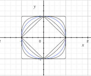
On \( \R^n \), we have a variety of norms, and hence a variety of metrics.
For \( n \in \N_+ \) and \( k \in [1, \infty) \), the function \( d_k \) given below is a metric on \( \R^n \): \[ d_k(\bs x, \bs y) = \left(\sum_{i=1}^n \left|x_i - y_i\right|^k\right)^{1/k}, \quad \bs x = (x_1, x_2, \ldots, x_n), \, \bs y = (y_1, y_2, \ldots, y_n) \in \R^n \]
Of course the metric \( d_2 \) is Euclidean distance, named for Euclid of course. This is the most important one, in a practical sense because it's the usual one that we use in the real world, and in a mathematical sense because the associated norm corresponds to the standard inner product on \( \R^n \) given by \[ \langle \bs x, \bs y \rangle = \sum_{i=1}^n x_i y_i, \quad \bs x = (x_1, x_2, \ldots, x_n), \, \bs y = (y_1, y_2, \ldots, y_n) \in \R^n \]
For \( n \in \N_+ \), the function \( d_\infty \) defined below is a metric on \( \R^n \): \[ d_\infty(\bs x, \bs y) = \max\{\left|x_i - y_i\right|: i \in \{1, 2 \ldots, n\}\}, \quad \bs x = (x_1, x_2, \ldots, x_n) \in \R^n \]
To justify the notation, recall that \( \| \bs x \|_k \to \|\bs x\|_\infty \) as \( k \to \infty \) for \( \bs x \in \R^n \), and hence \( d_k(\bs x, \bs y) \to d_\infty(\bs x, \bs y) \) as \( k \to \infty \) for \( \bs x, \bs y \in \R^n\).
Suppose now that \( S \) is a nonempty set. Recall that the collection \( \ms V \) of all functions \( f: S \to \R \) is a vector space under the usual pointwise definition of addition and scalar multiplication. That is, if \( f, \, g \in \ms V \) and \( c \in \R \), then \( f + g \in \ms V \) and \( c f \in \ms V \) are defined by \( (f + g)(x) = f(x) + g(x) \) and \( (c f)(x) = c f(x) \) for \( x \in S \). Recall further that the collection \( \ms{U} \) of bounded functions \(f: S \to \R \) is a vector subspace of \( \ms V \), and moreover, \( \| \cdot \| \) defined by \( \| f \| = \sup\{\left| f(x) \right|: x \in S\} \) is a norm on \( \ms{U} \), known as the supremum norm. It follow that \( \ms{U} \) is a metric space with the metric \( d \) defined by \[ d(f, g) = \| f - g \| = \sup\{\left|f(x) - g(x)\right|: x \in S\} \] Vector spaces of bounded, real-valued functions, with the supremum norm are very important in the study of probability and stochastic processes. Note that the supremum norm on \( \ms{U} \) generalizes the maximum norm in on \( \R^n \), since we can think of a point in \( \R^n \) as a function from \( \{1, 2, \ldots, n\} \) into \( \R \). Later, as part of our discussion on integration with respect to a positive measure, we will see how to generalize the \( k \) norms on \( \R^n \) to spaces of functions.
If we have a finite number of metric spaces, then we can combine the individual metrics, together with an norm on the vector space \( \R^n \), to create a norm on the Cartesian product space.
Suppose \( n \in \{2, 3, \ldots\} \), and that \( (S_i, d_i) \) is a metric space for each \( in \in \{1, 2, \ldots, n\} \). Suppose also that \( \| \cdot \| \) is a norm on \( \R^n \). Then the function \( d \) given as follows is a metric on \( S = S_1 \times S_2 \times \cdots \times S_n \): \[ d(\bs x, \bs y) = \left\|\left(d_1(x_1, y_1), d_2(x_2, y_2), \ldots, d_n(x_n, y_n)\right)\right\|, \quad \bs x = (x_1, x_2, \ldots, x_n), \, \bs y = (y_1, y_2, \ldots, y_n) \in S \]
Recall that a graph (in the combinatorial sense) consists of a countable set \( S \) of vertices and a set \( E \subseteq S \times S \) of edges. In this discussion, we assume that the graph is undirected in the sense that \( (x, y) \in E \) if and only if \( (y, x) \in E \), and has no loops so that \( (x, x) \notin E \) for \( x \in S \). Finally, recall that a path of length \( n \in \N_+ \) from \( x \in S \) to \( y \in S \) is a sequence \( (x_0, x_1, \ldots, x_n) \in S^{n+1} \) such that \( x_0 = x \), \( x_n = y \), and \( (x_{i-1}, x_i) \in E \) for \( i \in \{1, 2, \ldots, n\} \). The graph is connected if there exists a path of finite length between any two distinct vertices in \( S \). Such a graph has a natural metric:
Suppose that \( G = (S, E) \) is a connected graph. Then \( d \) defined as follows is a metric on \( S \): \( d(x, x) = 0 \) for \( x \in S \), and \( d(x, y) \) is the length of the shortest path from \( x \) to \( y \) for distinct \( x, \, y \in S \).
Suppose that \( S \) is a nonempty set. Recall that the discrete topology on \( S \) is \( \ms P(S) \), the power set of \( S \), so that every subset of \( S \) is open (and closed). The discrete topology is metrizable , and there are lots of metrics that generate this topology.
Suppose again that \( S \) is a nonempty set. A metric \( d \) on \( S \) with the property that there exists \( c \in (0, \infty) \) such that \( d(x, y) \ge c \) for distinct \( x, \, y \in S \) generates the discrete topology.
Note that \( B(x, c) = \{x\} \) for \( x \in S \). Hence \( \{x\} \) is open for each \( x \in S \).
So any metric that is bounded from below (for distinct points) generates the discrete topology. It's easy to see that there are such metrics.
Suppose again that \( S \) is a nonempty set. The function \( d \) on \( S \times S \) defined by \( d(x, x) = 0 \) for \( x \in S \) and \( d(x, y) = 1 \) for distinct \( x, \, y \in S \) is a metric on \( S \), known as the discrete metric. This metric generates the discrete topology.
Clearly \( d(x, y) = 0 \) if and only if \( x = y \), and \( d(x, y) = d(y, x) \) for \( x, \, y \in S \), so the positive and symmetric properties hold. For the triangle inequality, suppose \( x, \, y, \, z \in S \). The inequality trivially holds if the points are not distinct. If the points are distinct, then \( d(x, z) = 1 \) and \( d(x, y) + d(y, z) = 2 \).
In probability applications, the discrete topology is often appropriate when \( S \) is countable. Note also that the discrete metric is the graph distance if \( S \) is made into the complete graph, so that \( (x, y) \) is an edge for every pair of distinct vertices \( x, \, y \in S \).