
The Bernoulli trials process, named after Jacob Bernoulli, is one of the simplest yet most important random processes in probability. Essentially, the process is the mathematical abstraction of coin tossing, but because of its wide applicability, it is usually stated in terms of a sequence of generic trials
.
A sequence of Bernoulli trials satisfies the following assumptions:
Mathematically, the Bernoulli trials process with parameter \(p \in [0, 1]\) is a sequence of independent indicator random variables: \[ \bs{X} = (X_1, X_2, \ldots) \] each with the same probability density function: \[ \P(X_i = 1) = p, \quad \P(X_i = 0) = 1 - p \]
Recall that an indicator variable is a random variable that takes only the values 1 and 0, which in this setting denote success and failure, respectively. Indicator variable \(X_i\) simply records the outcome of trial \(i\). The distribution defined by the probability density function is known as the Bernoulli distribution. In statistical terms, the Bernoulli trials process corresponds to sampling from the Bernoulli distribution. In particular, the first \(n\) trials \((X_1, X_2, \ldots, X_n)\) form a random sample of size \(n\) from the Bernoulli distribution.
The joint probability density function \(f_n\) of \((X_1, X_2, \ldots, X_n)\) trials is given by \[ f_n(x_1, x_2, \ldots, x_n) = p^{x_1 + x_2 + \cdots + x_n} (1 - p)^{n- (x_1 + x_2 + \cdots + x_n)}, \quad (x_1, x_2, \ldots, x_n) \in \{0, 1\}^n \]
Note that the exponent of \(p\) in the probability density function is the number of successes in the \(n\) trials, while the exponent of \(1 - p\) is the number of failures.
If \(\bs{X} = (X_1, X_2, \ldots,)\) is a Bernoulli trials process with parameter \(p\) then \(\bs{1} - \bs{X} = (1 - X_1, 1 - X_2, \ldots)\) is a Bernoulli trials sequence with parameter \(1 - p\).
Suppose that \(\bs{U} = (U_1, U_2, \ldots)\) is a sequence of independent random variables, each with the uniform distribution on the interval \([0, 1]\). For \(p \in [0, 1]\) and \(i \in \N_+\), let \(X_i(p) = \bs{1}(U_i \le p)\). Then \(\bs{X}(p) = \left( X_1(p), X_2(p), \ldots \right)\) is a Bernoulli trials process with probability \(p\).
Note that in , the Bernoulli trials processes for all possible values of the parameter \(p\) are defined on a common probability space. This type of construction is sometimes referred to as coupling. This result also shows how to simulate a Bernoulli trials process with random numbers. All of the other random process studied in this chapter are functions of the Bernoulli trials sequence, and hence can be simulated as well.
Let \(X\) be an indciator variable with \(\P(X = 1) = p\), where \(p \in [0, 1]\). So \(X\) is the result of a generic Bernoulli trial and has the Bernoulli distribution with parameter \(p\). The following results give the mean, variance and some of the higher moments. A helpful fact is that if we take a positive power of an indicator variable, nothing happens; that is, \(X^n = X\) for \(n \gt 0\)
The mean and variance of \( X \) are
Note that the graph of \( \var(X) \), as a function of \( p \in [0, 1] \) is a parabola opening downward. In particular the largest value is \(\frac{1}{4}\) when \(p = \frac{1}{2}\), and the smallest value is 0 when \(p = 0\) or \(p = 1\). Of course, in the last two cases, \( X \) is deterministic, taking the single value 0 when \( p = 0 \) and the single value 1 when \( p = 1 \)
Suppose that \( p \in (0, 1) \). The skewness and kurtosis of \(X\) are
The probability generating function of \(X\) is \( P(t) = \E\left(t^X\right) = (1 - p) + p t \) for \( t \in \R \).
As we noted earlier, the most obvious example of Bernoulli trials is coin tossing, where success means heads and failure means tails. The parameter \(p\) is the probability of heads (so in general, the coin is biased).
In the basic coin experiment, set \(n = 100\) and For each \(p \in \{0.1, 0.3, 0.5, 0.7, 0.9\}\) run the experiment and observe the outcomes.
Recall that the Galton Board, named after Francis Galton, is a triangular array of pegs. The rows are numbered, from the top down, by \((0, 1, \ldots )\). Row \(n\) has \(n + 1\) pegs that are labeled, from left to right by \((0, 1, \ldots, n)\). So a peg can be uniquely identified by an ordered pair \((n, k)\) where \(n\) is the row number and \(k\) is the peg number in that row.
A ball is dropped onto the top peg \((0, 0)\) of the Galton board. In general, when the ball hits peg \((n, k)\), it either bounces to the left to peg \((n + 1, k)\) or to the right to peg \((n + 1, k + 1)\). The sequence of pegs that the ball hits is a path in the Galton board.
Recall also that there is a one-to-one correspondence between each pair of the following three collections:
So a sequence of \(n \in \N_+\) Bernoulli trials with success parameter \(p \in [0, 1]\) generates a random path in the Galton board with \(n\) rows, where \(p\) is the probability of a bounce to the right. In turn the trials also generate a random subset of \(\{1, 2, \ldots, n\}\), where each element is in the set, independently, with probability \(p\).
Open the Bernoulli Galton board experiment and set \(n = 20\). For various values of \(p\), run the experiment 100 times and note the Bernoulli trials, the paths in the Galton board, and the corresponding subset.
In a sense, the most general example of Bernoulli trials occurs when an experiment is replicated. Specifically, suppose that we have a basic random experiment and an event of interest \(A\). Suppose now that we create a compound experiment that consists of independent replications of the basic experiment. Define success on trial \(i\) to mean that event \(A\) occurred on the \(i\)th run, and define failure on trial \(i\) to mean that event \(A\) did not occur on the \(i\)th run. This clearly defines a Bernoulli trials process with parameter \(p = \P(A)\).
Bernoulli trials are also formed when we sample from a dichotomous population. Specifically, suppose that we have a population of two types of objects, which we will refer to as type 0 and type 1. For example, the objects could be persons, classified as male or female, or the objects could be components, classified as good or defective. We select \( n \) objects at random from the population; by definition, this means that each object in the population at the time of the draw is equally likely to be chosen. If the sampling is with replacement, then each object drawn is replaced before the next draw. In this case, successive draws are independent, so the types of the objects in the sample form a sequence of Bernoulli trials, in which the parameter \(p\) is the proportion of type 1 objects in the population. If the sampling is without replacement, then the successive draws are dependent, so the types of the objects in the sample do not form a sequence of Bernoulli trials. However, if the population size is large compared to the sample size, the dependence caused by not replacing the objects may be negligible, so that for all practical purposes, the types of the objects in the sample can be treated as a sequence of Bernoulli trials. Additional discussion of sampling from a dichotomous population is in the in the chapter finite sampling models.
Suppose that a student takes a multiple choice test. The test has 10 questions, each of which has 4 possible answers (only one correct). If the student blindly guesses the answer to each question, do the questions form a sequence of Bernoulli trials? If so, identify the trial outcomes and the parameter \(p\).
Yes, probably so. The outcomes are correct and incorrect and \(p = \frac{1}{4}\).
Candidate \(A\) is running for office in a certain district. Twenty persons are selected at random from the population of registered voters and asked if they prefer candidate \(A\). Do the responses form a sequence of Bernoulli trials? If so identify the trial outcomes and the meaning of the parameter \(p\).
Yes, approximately, assuming that the number of registered voters is large, compared to the sample size of 20. The outcomes are prefer \(A\) and do not prefer \(A\); \(p\) is the proportion of voters in the entire district who prefer \(A\).
An American roulette wheel has 38 slots; 18 are red, 18 are black, and 2 are green. A gambler plays roulette 15 times, betting on red each time. Do the outcomes form a sequence of Bernoulli trials? If so, identify the trial outcomes and the parameter \(p\).
Yes, the outcomes are red and black, and \(p = \frac{18}{38}\).
Roulette is discussed in more detail in the chapter on games of chance.
Two tennis players play a set of 6 games. Do the games form a sequence of Bernoulli trials? If so, identify the trial outcomes and the meaning of the parameter \(p\).
No, probably not. The games are almost certainly dependent, and the win probably depends on who is serving and so is not constant from game to game.
Recall that in the standard model of structural reliability, a system is composed of \(n\) components that operate independently of each other. Let \(X_i\) denote the state of component \(i\), where 1 means working and 0 means failure. If the components are all of the same type, then our basic assumption is that the state vector \[ \bs{X} = (X_1, X_2, \ldots, X_n) \] is a sequence of Bernoulli trials. The state of the system, (again where 1 means working and 0 means failed) depends only on the states of the components, and thus is a random variable \[ Y = s(X_1, X_, \ldots, X_n) \] where \(s: \{0, 1\}^n \to \{0, 1\}\) is the structure function. Generally, the probability that a device is working is the reliability of the device, so the parameter \(p\) of the Bernoulli trials sequence is the common reliability of the components. By independence, the system reliability \(r\) is a function of the component reliability: \[ r(p) = \P_p(Y = 1), \quad p \in [0, 1] \] where we are emphasizing the dependence of the probability measure \(\P\) on the parameter \(p\). Appropriately enough, this function is known as the reliability function. Our challenge is usually to find the reliability function, given the structure function.
A series system is working if and only if each component is working.
A parallel system is working if and only if at least one component is working.
Recall that in some cases, the system can be represented as a graph or network. The edges represent the components and the vertices the connections between the components. The system functions if and only if there is a working path between two designated vertices, which we will denote by \(a\) and \(b\).
Find the reliability of the Wheatstone bridge network shown below (named for Charles Wheatstone).
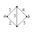
\(r(p) = p \, (2 \, p - p^2)^2 + (1 - p)(2 \, p^2 - p^4)\)
Suppose that each person in a population, independently of all others, has a certain disease with probability \(p \in (0, 1)\). So with respect to the disease, the persons in the population form a sequence of Bernoulli trials. The disease can be identified by a blood test, but of course the test has a cost.
For a group of \(k\) persons, we will compare two strategies. The first is to test the \(k\) persons individually, so that of course, \(k\) tests are required. The second strategy is to pool the blood samples of the \(k\) persons and test the pooled sample first. We assume that the test is negative if and only if all \(k\) persons are free of the disease; in this case just one test is required. On the other hand, the test is positive if and only if at least one person has the disease, in which case we then have to test the persons individually; in this case \(k + 1\) tests are required. Thus, let \(Y\) denote the number of tests required for the pooled strategy.
The number of tests \(Y\) has the following properties:
In terms of expected value, the pooled strategy is better than the basic strategy if and only if \[ p \lt 1 - \left( \frac{1}{k} \right)^{1/k} \]
The graph of the critical value \(p_k = 1 - (1 / k)^{1/k}\) as a function of \(k \in [2, 20]\) is shown in the graph below:
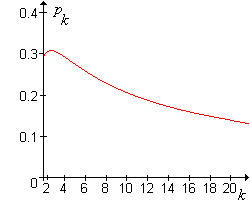
The critical value \(p_k\) satisfies the following properties:
It follows that if \(p \ge 0.307\), pooling never makes sense, regardless of the size of the group \(k\). At the other extreme, if \(p\) is very small, so that the disease is quite rare, pooling is better unless the group size \(k\) is very large.
Now suppose that we have \(n\) persons. If \(k \mid n\) then we can partition the population into \(n / k\) groups of \(k\) each, and apply the pooled strategy to each group. Note that \(k = 1\) corresponds to individual testing, and \(k = n\) corresponds to the pooled strategy on the entire population. Let \(Y_i\) denote the number of tests required for group \(i\).
The random variables \((Y_1, Y_2, \ldots, Y_{n/k})\) are independent and each has the distribution in .
The total number of tests required for this partitioning scheme is \(Z_{n,k} = Y_1 + Y_2 + \cdots + Y_{n/k}\).
The expected total number of tests is \[ \E(Z_{n,k}) = \begin{cases} n, & k = 1 \\ n \left[ \left(1 + \frac{1}{k} \right) - (1 - p)^k \right], & k \gt 1 \end{cases} \]
The variance of the total number of tests is \[ \var(Z_{n,}) = \begin{cases} 0, & k = 1 \\ n \, k \, (1 - p)^k \left[ 1 - (1 - p)^k \right], & k \gt 1 \end{cases} \]
So in terms of expected value, the optimal strategy is to group the population into \(n / k\) groups of size \(k\), where \(k\) minimizes the expected value function in . It is difficult to get a closed-form expression for the optimal value of \(k\), but this value can be determined numerically for specific \(n\) and \(p\).
For the following values of \(n\) and \(p\), find the optimal pooling size \(k\) and the expected number of tests. (Restrict your attention to values of \(k\) that divide \(n\).)
If \(k\) does not divide \(n\), then we could divide the population of \(n\) persons into \(\lfloor n / k \rfloor\) groups of \(k\) each and one remainder
group with \(n \mod k\) members. This clearly complicates the analysis, but does not introduce any new ideas, so we will leave this extension to the interested reader.